


In desperation I asked Fermi whether he was not impressed by the agreement between our calculated numbers and his measured numbers. He replied, “How many arbitrary parameters did you use for your calculations?” I thought for a moment about our cut-off procedures and said, “Four.” He said, “I remember my friend Johnny von Neumann used to say, with four parameters I can fit an elephant, and with five I can make him wiggle his trunk”.

So said Freeman Dyson, one of the brighter stars in the physics firmament. When we try to understand the star which supplies all the energy Earth needs to maintain life on its surface, we have a problem. The problem is it keeps surprising us with its unpredictable changes in activity levels. It’s doing this at the moment in solar cycle 24. The top solar physics institutions made various predictions about the timing of the start of the cycle, and how high the ampliitude would be. They’ve been proved very wrong. A couple of individual solar physicists did predict a low solar cycle (low for the modern era anyway), including Leif Svalgaard, who predicted a max monthly sunspot number of around 70 for this cycle back in 2004. Leif based his prediction on phenomenological observation of the solar polar field strength, which has been diminishing for a long time now. Even this is looking a bit high at the moment though. I predicted 35-50 SSN in 2008 based on a planetary method.
In this post, we take a cycles analysis approach to looking at solar activity since 1600. Regular contributor Tim Channon has done work in the past in acoustics, and as part of his toolbox, he developed some software which uses clever techniques to break down complex sound envelopes into underlying frequencies and amplitudes. For fun and interest, we fed it with the Lean 2000 TSI reconstruction data to see what would happen. The result is shown in the graph below the break.

The R^2 value for the correlation in the top graph between the Lean 2000 TSI reconstruction and the curve generated by Tim’s cycles analysis software is 0.99 – or in layman’s terms “Near enough perfect”.
The software decided to use seven cycles to get a best fit, and so following Johnny von Neumann’s metaphor, we were able not only to get Nellie to wiggle her trunk, but hold a brush with it and paint Lean’s TSI curve while doing a belly dance.
So, given the number of ‘arbitrary parameters’ to play with, this stuff is easy, right?
Well I haven’t seen anyone else manage it, so hats off to Tim Channon and his remarkable software.
Beyond that though, there is the question of whether there is any scientific value or merit in this kind of curve fitting exercise, or as Leif Svalgaard would have it, “cyclomania”. 🙂
It seems to me the answer to this depends on how ‘arbitrary’ the parameters really are. It has long been thought that the Sun’s activity and Earth’s climate exhibit some longer term cycles beyond the well known ~11 year Schwabe Cycle and the solar magnetic ~22 year Hale Cycle. There is also the ~80 year Gleissberg Cycle, and the ~200 year de Vries Cycle. There are also a couple more lesser known ones. The 55.15 year cycle identified by Roy Martin, and the ~110 year cycle noted recently by Roger Andrews in his SST vs Air temperature analysis. Roger notes in comments that not only is the periodicity right, but the phase is pretty close too.
Another point I want to stress here is that the cycles, which when combined reproduce the Lean TSI curve so perfectly, were not ‘picked’ by a human with pre-conceived ideas or knowledge of real natural cycles in terrestrial climate or solar activity. The software did the choosing, testing and refining all by itself.
Look again at the legend at the bottom of the lower graph, where the frequencies of the cycles Tim’s software found are enumerated:
11.09, 11.51, 57.2, 78.94, 112.5, 238.86, 426.47 years.
Most of these are close to periods recognised by solar physicists, climatologists and planetary cycle periods identified by researchers here on this blog.
Given that the Lean TSI reconstruction is no doubt imperfect, there remains the question of how a curve generated by nearby exact planetary synodic frequencies would look compared to it. This is a project I’ll be undertaking soon.
What happens when you project the synthesized curve further backwards and forwards in time?
Watch this space, it’ll be worth your time, I promise.

Interesting. Any significance to all of the waves trending down at once, as the graph shows them doing now?
Tallbloke and Tim:
Congratulations. I’ve been messing around for years with maybe a dozen arbitrary parameters and I’ve only just managed to find the elephant.
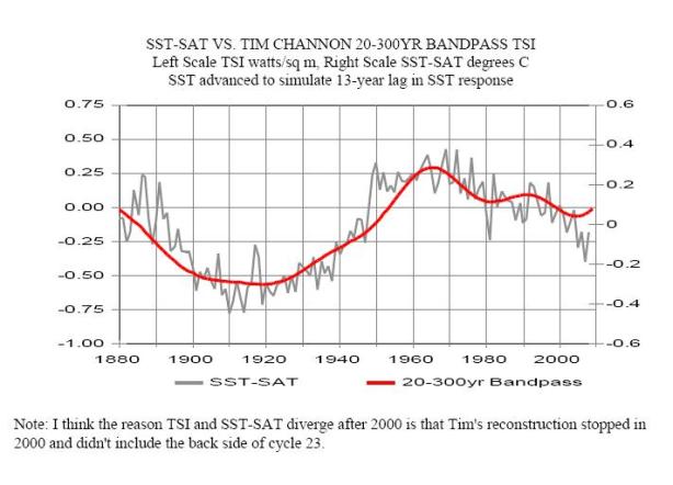
The 112.5 year cycle plotted in your second graph matches the +/-110 year cycle in SST-minus-SAT with no significant phase shift. However, your +/-11 year cycles don’t seem to have been plotted in this graph, and as far as I can see the Schwabe-cycle oscillations in the reconstruction aren’t a heterodyne effect. These oscillations are also much larger in the 19th century than in the 20th. Any reason for this?
“Beyond that though, there is the question of whether there is any scientific value to this kind of curve fitting exercise.” Well, according to my phenomenological model results your curve-fitting just generated about 0.8C of natural cooling between now and 2050, and I would trust this estimate at least as much as I trust any of the IPCC’s models.
WOW, we are at 2010 and it is on curve. If this proves out you now have a tool that will let you check the various inputs to see their effect or lack thereof on interplanetary effects and timing on solar output. Maybe then we can tease magnatisim from gravity. pg
After further study, questions; can the individual waves be modeled? The earth / moon pair is a complex thing both in gravity and magnetics. The modeled TSI shows flattening 1920 and later. Wonder what it will look like with real numbers. Great anticipation here. First the sun and then the world! 😎 pg
Oh, my! Wheels within wheels! Will be watching with great interest. Thanks for this.
Many years ago I worked on Decca Navigator radio stations. Those curves rang my bell. 🙂
Bob: Only two out of the seven waves are trending down strongly at the moment. Three are just peaking and will soon be falling, and the two shorter cycles which aren’t shown are partially cancelling each other.
Are you asking about significance in terms of the way the software handles it’s job or significance in terms of the climate implications if the combining curves are representative of reality and the Sun has a strong effect on climate?
Roger: Tim is the star of the show here. I’m just the person ‘putting it out there’ and commenting on the potential significance of the match between the composing curves and real cycles in nature.
“I would trust this estimate at least as much as I trust any of the IPCC’s models”
Damned with faint praise. Lol. Why don’t you ask one of the IPCC modelers to try running their model from 1610…But that’s not really fair, or is it?
It’s true that the software struggled to replicate the ~11year solar cycle amplitudes consistently, more to be done here clearly. I think other techniques like the one Roy Martin developed may help, in conjunction with Tim’s software output.We didn’t show the curves because they would have cluttered the graph and anyway we know them not to be ‘real’ as a combination. The mid-long term periodicities lying nearer the middle and outer edges of the envelope are the most important here.
I’d be very cautious about putting a figure on the potential fall in global surface temperature at the moment. My simple solar-planetary model which uses integrated sunspot numbers as a proxy for ocean heat content cushions the effect of a sudden TSI drop. Plus, the oceans tend to burp out excess energy stored during runs of high solar cycles when the sun quietens down, and this will help maintain SST’s and air temps. There is much to learn in this area too. If the model is right, and the data we get from ARGO is honest and produced in a way unbiased by preconceptions, we will see a significant drop in Ocean Heat Content proportional to our generated curve.
P.G.: Some tweaking can be done, but the software deals in sine waves only at the moment. There is much to discover just with sine waves though, so I’m not too worried about this.
Richard: Yes. Like carrier waves. Intriguing isn’t it? I’m sure Tim will stop by to tell us a bit more about the software soon, though he has a lot on at the moment. Any scientists who want their datasets analysing should contact me in the first instance.
Well done.
– If TSI is the governor of global temperature then + – 1.5W/m2 is not going to do great deal for either the global warming or cooling.
– You need to back extrapolate to 1000AD, to see how it fares against other SSN grand minima.
– If it does, than the hardest part is to find source of the frequencies involved, and show that there is an acceptable physical mechanism.
When done you’ve arrived !
Hi Vuk, and thanks for your input, valid points all.
Nir Shaviv found that the solar variation is amplified 7-10 times by terrestrial mechanisms in his JGR paper on using the oceans as a calorimeter. He didn’t state what they are for certain, but the guess I’d go with is magnetism and it’s effect on clouds via your hypotheses and the Svensmark effect as the big one. Knutti found that the climate sensitivity might be higher once the way heat is transported from equator to poles is factored in properly.
I’ll be putting up a post showing how the output looks when we go back as far as the Roman and Minoan warm periods soon. First I want some discussion on validity and some ideas about potentially useful periodicities.
NASA scientists Wolff and Patrone have a potentially viable mechanism for the effect of the planets motions on solar variability. Demonstrating that with time series is another project in progress. The frequencies are the puzzle, and your equations provide some of the keys to unlock the solution. Please come with us on the journey so we can all arrive together.
Milankovitch cycles were also rejected as a cause of the ice ages because the calculated total energy change was not enough. What is ignored in climate science is that cyclic behavior is self amplifying.
Think of a child on a swing. A small signal repeated in phase gives rise to a large observed motion. This is how the tides work on earth. The forcing is quite small, but because it is cyclic it leads to large observed motion in some spots on earth, and in other spots there is almost no motion.
This is what is ignored in climate science. That cyclic forcings are likely to lead to large regional changes in climate in some spots on earth, and small chanes in other spots. By treating climate as an average they have totally missed the plot.
A study of the tides is quite revealing because they are much more complex than one might imagine, yet they are quite predictable using just the sort of analysis you are doing for TSI.
Yes, you would have to model the earth and then the moon as two concurrent sine waves, one over the other so that you would have a traveling spike, tricky that! At least there is only one pair that is significant to the sun and it may be too small to see gravitationally. Magnetic effects may be more pronounced due to shading. pg
ps: I forgot to add that the problem for many people is to think in terms of cycles many times longer than human lifetimes. They find it hard to imagine that a pendulum doesn’t care how long it takes to swing back and forth. To a human being, if a pendulum has a period in excess of 100 years it is extremely difficult to prove that the motion is cyclic. At any point in time the motion will look linear. If the period of the pendulum is 100 k years, then for all intents and purposes, it will appear that the pendulum is not moving. Measuring the motion and proving that it is cyclic is almost impossible, unless there is a geological record to match.
“Yes, you would have to model the earth and then the moon as two concurrent sine waves”
That is a good approximation. The orbits follow longer cycles as well which must be taken into account. Then you need to acount for regional differences caused by the shape of the ocean basins. If you averaged the tide globally you would miss this. See fig 4 on the URL below.
http://en.wikipedia.org/wiki/Tide
This is likely a great deal to be clearned about climate by using the tides as a model. For example, these quotes from Wikipedia:
“The theoretical amplitude of oceanic tides caused by the Moon is about 54 centimetres (21 in) at the highest point.” … “The Sun similarly causes tides, of which the theoretical amplitude is about 25 centimetres (9.8 in)”
Where I live, a 10 foot tidal range is common. In Darwin Australia we experienced regular tides of 25 feet. Cyclic forcings create much larger motion than is predicted by naive application of theory.
This is also from Wikipedia:
“The tidal force on a particle equals about one ten millionth that of Earth’s gravitational force.”
So, maybe a 1.5 W/m2 TSI difference is more significant than it might first appear? After all, one part in a ten million difference in the gravitation force moves one heck of a lot of water.
Tallbloke: You do me unjust. I wasn’t damning with faint praise – I was praising with faint damns. I just forgot to put the faint damns in.
Re heat retention in the ocean. Since I read your earlier post on integrating SSN>40 I’ve been trying to come up with empirical evidence to support the idea that solar heat builds up at the ocean surface above a certain threshold level and over long periods of time, but I haven’t been able to find any. I can still fit SST to solar only when I assume a transient SST response to solar forcing with a +/- 12 year lag in SST.
And if the SST response to solar forcing is indeed transient, and if your TSI projection is reasonably accurate, and if my phenom. model is somewhere close to reality, then we are indeed going to get about 0.8C of solar-induced SST cooling between now and 2050. (The IPCC will of course insist on adding an AGW component, but I don’t think it would be this large.)
Here’s a new twist on your theory. Solar heat does accumulate in the ocean during periods of high solar activity, but at depth, not at the surface. (We need some kind of a downward heat transport mechanism to explain the cyclic SST-SAT relationship anyway.) Any thoughts?
Hi Roger,
I’ve always thought the excess energy must be forced down into the ocean. There is nowhere else for it to go. What gave you the impression I was talking about accumulation of heat at the surface? My point about the way the solar effect on climate is underestimated is due to the energy disappearing to places where we weren’t measuring it.
Mechanisms for downward transport. I asked Judy Curry and Peter Webster about this at Lisbon as we toured the castle walls. They said plenty of overturning and mixing to much greater depths than the tropical thermocline is achieved by cyclones, tides and currents. Add to those the basin sloshing induced by changes in Earth’s length of day, and the currents altered by 18.6 year lunar declinational cycle and there is plenty of mobility for energy transport in the oceans.
Having said that, there is plenty we don’t know about this stuff, so attacking it from all angles seems a good move. Thanks by the way GE and P.G. for your comments on tides.
A random thought. I don’t know what Tim Channon’s profession is, but he seems to have done all this wearing an acoustical engineer’s hat. Clearly climate science is too important to be left to the climate scientists.
“Solar heat does accumulate in the ocean during periods of high solar activity”
I spent 20 years sailing offshore and would certainly agree with that, though it can be surprisingly cold on the deep oceans even right on the equator. Shallow areas like Indonesia where the water is 200 feet deep for thousands of square miles the water temperature does heat up.
A mechanism to move heat from the surface to the deep oceans? Sure, consider the wind. As warm surface water moves as a result of wind and tides it will force slighty cooler water downward, and colder water at the bottom of the ocean will flow like a river to make room for the water.
In those places where the warm water has left, slightly cooler water will rise to take its place, and the cold river at the bottom of the ocean will flow into the space made available.
The problem in visualizing warm water sinking is in assuming that water is stationary. It isn’t. Surface water on the open oceans moves about 15-30 miles per day, sometimes a lot more. That is a huge volume of water in motion with a lot of thermal energy. Somewhere there has to be water rising and sinking to make room for this motion, with a lot of thermal energy travelling vertically.
This is historic. The Magister Ludi´s Academy working !. Now as M.Vukcevic says: ….If it does, then the hardest part is to find [the] source of the frequencies involved, and show that there is an acceptable physical mechanism…
I couldn´t dare as I am just a layman, but who dares?
That finding would be an epiphany.
Tallbloke: What gave me the impression you were talking about accumulation of heat at the surface was your comment: “I’d be very cautious about putting a figure on the potential fall in global surface temperature at the moment. My simple solar-planetary model which uses integrated sunspot numbers as a proxy for ocean heat content cushions the effect of a sudden TSI drop.” My point was that while there would be a cushioning effect relative to OHC there wouldn’t necessarily be one relative to global surface temperature, which is what I was predicting (projecting?). Anyway, apologies for misinterpreting you.
Amazing, incidentally, that we still don’t have an accepted metric for measuring global warming.
Thanks Tim, that’s a very revealing plot. My own view on this is that the de Vries solar quasi-cycle of 210y(ish) seems to have had the main impact as shown in the (poor) historic record.
The cycle seems to cause 100y(ish) periods of regular cooling and warming but never with good correlation at the decadal scale. There always seems to be periods of warming within the cooling half of the cycle and periods of cooling within the warming half of the cycle so a definite pattern is hard to see. The amplitude and length of the max. cool or max. warm period within each half quasi-cycle also varies quite a lot.
Perhaps the other longer and shorter term over-lapping quasi-cycles smear the signal due to the deterministic chaos inherent in our climate system. I’m concerned that we are just at the start of the cooling half quasi-cycle and are already seeing colder NH winters in areas of dense population. It could be that what history shows us are regional effect, with very cold winters in China, USA and Europe.
Maybe the greater proportion of sea in the SH buffers the change and they get more normal winters, but cooler summers. I don’t think the long-term records are good enough to show this.
Average climate is a useless concept. It’s what is happening where people live that’s important.
“My point was that while there would be a cushioning effect relative to OHC there wouldn’t necessarily be one relative to global surface temperature”
Ah, well, you haven’t read enough of my ramblings on this subject. My hypothesis is that the heat forced down into the ocean when the Sun is more than averagely active comes back out again when the Sun is below par. This is why you get big el nino’s near solar minimum. There has been one at the last five solar minima. So energy rises back to the surface, warming the SST’s and depleting the OHC as it convects and radiates to the atmosphere. The Ocean Heat Content is the correct metric for global warming/cooling if you are trying to understand the energy flows in the large. You need to do this in order to understand solar input, and the lag which masks the size of the solar signal in the Earth’s climate. Because big el nino’s at solar min and la nina’s at solr max flatten the signal in surface measurements.
Tenuc:
“Average climate is a useless concept. It’s what is happening where people live that’s important.”
Well that’s what is important to farmers and the people who eat their produce. For the climatologist, an understanding of the energy transfers under the ocean surface is essential if you’re going to be able to work out which the important climate factors really are. If you don’t manage that, you’re not going to be able to make useful predictions the farmers can improve their chances of good crops with by being able to better plan for the future.
Back in the days of dinosaurs, I was at university in a poorly remembered astronomy program. I recall a “Fourier” analysis of complex frequency patterns to deconstruct them to their component, simple frequencies. Is this different? And why hasn’t such a wave-deconstruction program been run before? I’m sure mechanical engineers specializing in vibration problems do this regularly.
“My hypothesis is that the heat forced down into the ocean when the Sun is more than averagely active comes back out again when the Sun is below par”
This makes perfect sense to me. A change in the vertical temperature gradiant perhaps combined with a change in wind strength controls when the cold deep ocean river is able to break out at the surface. Otherwise it is trapped below where it forms a lake of cold water as the cold river of water continues to flow and pressure builds. Once conditions are right this lake breaks out and overflows at the surface, to produce alternating el nino, la nina effects.
Doug, from what I understand, that is what the software does. It creates Fourier analyses on the fly and refines the cycles until the best match is achieved. I don’t know why it hasn’t been run on solar data before, but I’m glad Tim got the ‘Talkshop Team’ there first!
” For the climatologist, an understanding of the energy transfers under the ocean surface is essential if you’re going to be able to work out which the important climate factors really are.”
If you average things out, there is probably very little net energy transfer. For example, if you averaged the tides over a year, the motion is negligible.
The reason Climate Science averages things out is not to increase understanding, it is because the volume of data is too large to manage otherwise. However, averaging decreases the information available, which can lead to false conclusions.
ge0500, yes, and also, a colder clearer atmosphere loses heat to space faster and so cools quickly, creating a bigger temperature differential with the sea surface. This permits energy to move more quickly from the ocean to the atmosphere, and out to space. The question is, how fast does it deplete OHC? It looks like we’ll start finding out over the next few years and I’ll be able to refine my simple solar-planetary energy model.
tallbloke says:
February 21, 2011 at 5:11 pm
“Tenuc:
“Average climate is a useless concept. It’s what is happening where people live that’s important.”
Well that’s what is important to farmers and the people who eat their produce. For the climatologist, an understanding of the energy transfers under the ocean surface is essential if you’re going to be able to work out which the important climate factors really are. If you don’t manage that, you’re not going to be able to make useful predictions the farmers can improve their chances of good crops with by being able to better plan for the future.”
I agree Rog, but because the system is dynamic, it is not enough just to know the average thermal global energy in the system. You need to know where the energy is being stored or discharged at each moment in time and how it gets moved about to different places on the globe. Only by understanding the detail of how the system responds geographically to small changes in solar energy input of all types can useful regional predictions be made.
Climate science seems to have forgotten that averaging the behaviour of a non-linear dynamic system ,like our climate, provides little or no information about likely future events.
Tallbloke, if you haven’t encountered Ray Tomes, go to http://ray.tomes.biz/ and do it. If anyone can help out with cycles, he’s the man – he’s been studying them for years.
Cyclical processes do seem to me to be much more likely as an explanation of the climate’s workings than the accumulating effects of a trace gas (mind you, I’ve visited Mr. Tomes’ website myself 😉 I’ll be interested to see if you can correlate the cycles with known phenomena – that’s got to be the nitty gritty.
Hi Steve, and welcome.
As it happens I emailed Ray this morning and reposted this post in draft form on the Cycle Research Institute website. 😉
I agree that finding the right cycles in nature and matching them to the analysis is the big challenge. I’m pretty sure we are missing a few in this analysis. One of around 900 years and another at around 2350 years. probably another at around 4600 years too but that one isn’t too important for our timeframe in this interglacial.
The research continues…
Forget cycles for few minutes, sit back and enjoy celestial fireworks (keep an eye for comet in March, Halloween and Christmas displays.
http://www.youtube.com/watch_popup?v=dvBI4Kirpbw&vq=large
I’m at a bit of a loss on what to say without a mountain of information, either overload or bore.
“tallbloke says:
February 21, 2011 at 5:23 pm
Doug, from what I understand, that is what the software does. It creates Fourier analyses on the fly and refines the cycles until the best match is achieved. ”
That is a good description as a kernel of the concept. Lots of different ways of describing it but one that clicks with you the reader is the hard part.
A normal Discrete Fourier Transform DFT is an approximation and ambiguous. It cannot give accurate numbers for frequency, amplitude or phase. It is possible to interpolate but this is still not very good.
In essence I am creating an FT from discrete in time data: the numbers are not quantised by bin etc. On other kinds of problem it spits out somewhat accurate data measurements.
The number of terms used is limited, kind of principle components.
I can for example derive a model of Mauna Loa CO2 hourly data 1958-1986, r2=0.996 using 3 terms. If this model is changed to monthly, forecast 23 years to date and compared with published monthly data, r2 = 0.998
The whole period 1958 to 2011 error is <+-4ppm
Satellite sea level data was found to be strongly predictive, story in there.
Solar data is hard and the path forwards continues.
Solar, temperature, sea level connected? Yup but without a mechanism this is just a curiosity.
The output is a model of the data and includes a ready for spreadsheet import model which can be rebased to different time quantisation etc.
Another important tool is end corrected filtering.
What Tallbloke has shown has not had any work done on predictability, often a lot of work. Results range from law through to forget it, is either random or not understood.
There is another way of working on the Lean data, can be decomposed by filter and Tallbloke has seen a result but I asked he didn't publish. Reason: whilst it is rational it is also not stable enough to draw the conclusion I think we wish was there. I don't want to get labelled as a lune. (can do that myself)
If there is genuine interest I will see if a compromise can be shown in this thread.
I concluded that Lean does not disagree with that interpretation but neither is it a safe conclusion.
Tim, thanks for the comments and notes. Definitely still a work in progress, and you’re right to emphasise that. The result is still too good not to share though. 🙂
Hopefully, some further ideas will come out of comments here which will be usefull in firming up the basis for this approach.
Well I haven’t seen anyone else manage it, so hats off to Tim Channon and his remarkable software
This graph must be kept as a bookmark. It is not only about that small climate thing it´s cycles.
Tim; can you input a frequency or more and then instruct the program to find the other frequencies to get the base match or does it only look for the harmonics to the match the base? pg
Re cycle lengths 11.09, 11.51, 57.2, 78.94, 112.5, 238.86, 426.47 years, the first two match the Schwabe and Hale cycles, and the third is close to the Jupiter-Saturn tri-synodic cycle (59.58 years). The longer cycles, however, do not match the Gleissberg (90 years) or De Vries (210 years) solar cycles or the Jose planetary cycle (178.7 years):
http://solarimg.org/forum/viewtopic.php?f=6&t=126
The above is not in any way intended to diminish the value of Tim’s analysis. Planetary analysis should take a back seat to other methods, if those other methods produce results that turn out to better match hard observational data.
Unfortunately, the only really good solar data is satellite data from 1979 to present (less than three normal Schwabe cycles, or 1.5 Hale cycle). In that time frame, the Sun is behaving very unpredictably.
A variety of things are possible PGS and if not it is my source code.
There is no magic bullet so please don’t expect much.
Normal operation in involves a few command parameters and wait. It decides on where to start and what to add. Just the sample rate and how many terms to use plus the input file. Things can of course be more complex.
What you want might be escape out, edit in some specific data, lock most things and resume. When it has settled (roughly sorted out phase and amplitude), stop and take off the locks, resume.
This where it is all a human call, no way of knowing what will happen.
Looking at the input data is a good idea, including the spectrum. With this long period data there is often little information but spectral broadening can give clues on what the structure might be, is beyond that kind of analysis.
A spectrum of the residual shows what is remaining.
Gerry: A great deal needs to be said and discussed about periodic factors. I am afraid that a lot of what is written has no basis, things do not combine in the patterns supposed. Action at a distance does vector sums.
That said and tends to be dismissive of eg. gravitational effect, it does not follow that eg. speed of light magnetic effects are not planet positional effective. I think very little is known about solar system magnetic and similar factors. This is of course linked to the cosmic ray problem.
Don’t take any of this as a conversation stopper, I can be wrong and do make mistakes.
Kind of an aside. Was looking through the NOAA archive.
I came across some pretty much sick stuff from history, are a joke, but one item took my attention, Overpeck paper from 1998.
This is about Arctic and includes a version of Lean. Pull that up and look in case it is significantly different, nope. Casually chucked to though a 100 year filter, no surprise.
Also so in the data is a temperature dataset over the same period. Pull that out and hurl it through the same filter. Plot both.
Wicked thought, I wonder if. Scale and offset the temperature data, just ax+y
Oh dear, it is very close to a clone of the Lean.
Read supporting text
“Abstract
A compilation of paleoclimate records from lake sediments, trees, glaciers,
and marine sediments provides a view of circum-Arctic environmental variability
over the last 400 years. From 1840 to the mid-20th century, the Arctic warmed to the highest levels in four centuries. This warming ended the Little Ice Age in the Arctic and has caused dramatic retreats of glaciers, melting of permafrost and sea-ice, and alteration of terrestrial and lake ecosystems. Although significant warming, particularly after 1920, was likely due to increases in atmospheric trace-gases, the initiation of the warming in the mid-19th century suggests that increased solar irradiance, decreased volcanic activity, and feedbacks internal to the climate system played roles.”
So why is the temperature a clone of the solar TSI you show? Seems a move along, nothing to see here.
ftp://ftp.ncdc.noaa.gov/pub/data/paleo/paleocean/by_contributor/overpeck1997/
Some really useful contributions here that have jogged some ideas about how to advance this technique, thanks everyone.
Following up P.G.’s question and Tim’s reply, and Gerry’s timely admonition regarding the short length of reliable data. I also got an email back from Ray Tomes last night pointing out the timescale the limit of accurate spectral analysis given the length of the base data.
I was wondering if it might be possible to build several proxy datasets using ‘the best we’ve got’. i.e. splice up the datellite TSI with suitable Maunder onwards reconstructions such as Lean’s and Svalgaards, and tack on the paleo and 10Be stuff beyond that all the way back to the year dot.
The Ljungqvist 2010 curve lgl posted on the 10Be thread might be worth a try.
Although we’d expect the result to be ‘through a glass darkly’, it might tighten the longer cycles up and give us a better idea of whether the simpler planetary relationships are operative, or whether we are looking at a complex mix of gravitational and electromagnetic influences. Or something else entirely.
We should remember the interesting result Gray Stevens turned up at this point which seemed to indicate maxima in solar activity occurred when there is a lineup of big planets both in straight line gravitational terms and along the parker spiral. More analysis is needed there to see if that configuration consistently has an effect. Problem is it is so rare there are not many examples to test against the sunspot record.
Regarding the de Vries cycle; are there any proxies going back a long way which show a really regular tight 210 years?
Tim has sent me another spreadsheet he’s produced with the following graphs included.
I’ll let Tim do the ‘splainin 🙂
I’ll just note that the peak to peak on the blue curve matches the period Semi identified for the cycle of total angular momentum in the solar system. If I recall correctly he re-calculated it to be around 934 years. Tim didn’t know about that in advance so this is a very pleasing result.
This is comment number 42. Heh. 🙂
“Following up P.G.’s question and Tim’s reply, and Gerry’s timely admonition regarding the short length of reliable data. I also got an email back from Ray Tomes last night pointing out the timescale the limit of accurate spectral analysis given the length of the base data.”
That is not purely true, needs more context on what it means. This is not a criticism of Ray who would have been briefly answering a question without knowing the full context.
I am pushing the envelope by using indirect computation by (in essence) shape matching, whereas a direct spectral analysis and particularly on discrete data cannot even go as far as what Ray Tomes says. More bluntly it cannot compute _any_ spectral line, merely there is a line (frequency) somewhere between the frequency bin (as in notional container) lower and upper boundary. Similarly phase and amplitude have serious limitations on accuracy.
The above applies to the largest (quantity sense) DFT which can provide more information, which is the smallest bin size.
In essence I am refining to an FT using Discrete (sampled) data. This will also be trading on quantisation, which for the kind of data involved is woefully poor.
That is partly why I am trying to be cautious. This is one of the fun areas, heuristics where there is no pure answer. Not dissimilar to the chess playing computer and with the better example of the travelling salesman problem, a problem where for significant but surprisingly small N it cannot be computed in a sane length of time.
Heuristics can provide an engineering solution. Do you want a good answer or none?
Think I am kidding?
Give me the data for a sensible fragment and I’ll see what happens and show you. This can be audited if there is dispute and Tallbloke has a copy of the program as a reference.
I expect there are ‘net texts explaining but no good ones come to mind.
Real people discussing where it might or might not be accessible is here, very useful site
http://www.dsprelated.com/showmessage/108339/1.php
Companies like this one tend to write from the position of actually doing for real
http://www.bores.com/courses/advanced/windows/10_kern.htm
Otherwise try a ‘net search and if you discover something clear let us know. As so often it can be the very devil explaining an idea or concept to another person. In this example a ‘net trawl shows a working history of explanation attempts, elliptic answers, daft questions, wrong, you name it.
Using only the strongest components of the spectrum you get the longer cycles ‘for free’ looking at the envelope. http://virakkraft.com/SunspotFFT.jpg (far from perfect but I didn’t attempt finetuning amplitude and phase)
Re: comment 42, monkey man. 🙂
The very long period is ambiguous. Something is thereabouts, a lovely old word.
Neither will reality be a precise math shape, be knobbly and wobbly.
The point is that the human record says something akin to that is history, so this is consistent with that but it is not a solid proof. In private where there is trust and knowledge that ideas are being banged about showing such things is rarely a problem. In public is a whole different kind of fish.
I’d shown something similar to Tallbloke in private where his reaction was wanting to show it, I objected precisely because this is asking for a cold shower from others.
Tim Channon says:
February 22, 2011 at 10:52 am
Great comment Tim and needed to be said. I think this issue is a major problem in finding truth, and leads to the sort of confirmation bias seen across the whole of modern science. Only fluff which matches the current paradigm is allowed to pass through the gate of the peer review process, while anything which would falsify the mainstream ideas is blocked, or attempts made to destroy it.
For example, most of the paleo temperature data-sets are lacking in spacial sampling points and suffer from incorrect assumptions about how proxies respond to change. Even current data-sets have some of these issues and the temperature record ends up smeared and imprecise. It ends up like looking through a telescope with the lens covered in Vaseline – add as many layers of dust to this as you like as we go further back in time.
Tim,
Constructive criticism is always welcome. This site provides a waterproof and fire retardant umbrella for those discussions which otherwise attract hosers, flamethrowers, and other assorted impolites.
There is nothing wrong with discussing conjectural possibilies, provided they are not put forward as fully formed theories with high levels of certainty.
I’m past caring about the posturings of people who are more guilty of peddling guesses as solid science than we are. Let them rant while we get on with the pursuit of knowledge.
The 934 years is the approximate centre of an envelope which probably ranges from about 870-960 years. The motion of the planets taken as an ensemble never repeats exactly on any timescale. That’s part of the fun in working out the puzzle. I’m trying to achieve good engineering estimate, not perfection which doesn’t and can’t exist. This is the ‘partially deterministic chaos’ Tenuc talks about.
@lgl. Thanks for sharing. What does the bottom edge of the graph look like?
Tallbloke
The buttom envelope is a mirror of the upper. Using 10 and 11 yrs is just a ‘trick’ to avoid using the real cycles (Ju-Sa 20 yrs and Ju-Ea-Ve 22 yrs) and then rectify like nature does. Perhaps Tims software can do it the proper way. Not sure whether the 11.8 Ju cycle should be kept or made 2*11.8.
[Edit] Understood, thanks.
Tallbloke/Tim:
Hi. Any chance of getting the numerical data for “lean split into 3 components” graph you showed earlier?
[edit] Almost certainly not a problem. Courtesy check with Tim first.
tallbloke says:
February 22, 2011 at 11:46 am
“…I’m trying to achieve good engineering estimate, not perfection which doesn’t and can’t exist. This is the ‘partially deterministic chaos’ Tenuc talks about…”
That’s the best anyone can do. The accuracy possible for prediction of future events depends on data/knowledge of the past, the non-linearity inherent in the system and our ability to identify random ‘black swan’ events. A ‘good engineering estimate’ is still useful in that it allows focus to be directed on the part of our complex system likely to deliver the low hanging fruit. Shame the IPCC climate scientists cherry-picked CO2 as the main driver of change, rather than looking up to the stars.
This is a short but revealing quote from the ACCRIM website:-
“…TSI proxies during the past 400 years and the records of surface temperature show that TSI variation has been the dominant forcing for climate change during the industrial era. The periodic character of the TSI record indicates that solar forcing of climate change will likely be the dominant variable contributor to climate change in the future…”
http://www.acrim.com/
Looks like at least some mainstream scientists still have stonking big hairy balls… 🙂
Tenuc,
Yes, Richard WIlson, ACRIM P.I. and Nicola Scafetta ACRIM team member and author of several bullseye papers including the rebuttal of the Gavin Schmidt et al solar paper a couple of years ago. Google Scafettas rebuttal on Pielke Seniors site, a fun read. So is the Climate audit thread. 😉
Read this too.

from Old Goat’s Almanac
Leif Svalgaard says:
February 21, 2011 at 4:50 pm
tallbloke says:
February 21, 2011 at 3:15 am
the new solar forecasting technique outlined on my blog is forecasting a four decade drop in TSI…
Based on physical considerations [not cyclomania 🙂 ],
I tend to think that SC25 will be larger than SC24, possible significantly higher.
Vuk,
Lol. Replied:
tallbloke says:
February 22, 2011 at 7:55 am
Nice to see a smiley in there Leif. Good on you for making a prediction too. 🙂
Vuk: If those cycles (waves), represent energy, of how much energy are we talking about?
As you said:…then the hardest part is to find [the] source of the frequencies involved, and show that there is an acceptable physical mechanism
My guess is that you can tell us more.. 🙂
RA sure. Just a matter of agreeing who, what and how. It is Tallbloke’s place.
lgl: I think you could do that using ephemeris software or from data it outputs.
Adolfo Giurfa says:
February 22, 2011 at 4:10 pm
“Vuk: If those cycles (waves), represent energy, of how much energy are we talking about?
As you said:…then the hardest part is to find [the] source of the frequencies involved, and show that there is an acceptable physical mechanism
My guess is that you can tell us more.. :-)”
Good question Adolfo. The IPCC cabal of CAGW scientists speculate that a doubling of a trace gas could have a big effect, unlikely as that sounds.
It could be that only small amounts of energy need to change, which are amplified by changes to albedo, ocean current, winds etc. When driving my car, just a few ounces of pressure on the accelerator unleashes 225bhp, which then catapults the car down the road with great speed.
Tallbloke and Tim: Thanks for the data. The 25-300yr bandpass plot (red line) on the “Lean split into three components” graph you showed earlier is an excellent fit to the SST-SAT graph I showed in the “plot thickens” thread, allowing for a +/- 13 lag in SST-SAT response.
Roger, Good spot!
So you think this makes the case for solar influence on SST SAT relationship a lot stronger than before? Doesn’t look like there is a lot of room left for anything else to me.
The temporal location of the inflection point is interesting too. But this decline isn’t hidden. 😉
Tallbloke:
The way I see it is this. Tim is sitting in front of his computer applying harmonic analysis to the TSI record to see if he can project future solar activity. He doesn’t know I exist. At the same time I’m sitting in front of my computer thousands of miles away messing around with temperature records to see if I can find a relation between SST and air temperature. I don’t know that Tim exists either. Now we put our results together and get a +/-0.9 correlation. There’s always the chance that this could be serendipity, but I don’t think it’s very likely.
Roger,
Welcome to the undefinable magic of the Talkshop.
🙂
Roger A: Need to sort that out, it was a casual, wasn’t treating the dataset particularly seriously. On the other hand so much has gone nuts since 200x anything is possible.
I think you have the lot including the input data. Not neat and tidy, column E is the Lean data and yes it stops at 2000. Ah got it, must be Y2K problem.
Serious: bandpass is column D with no data after 2000.
Umm… so what is going on? Is your plot software ignoring missing data?
I can incidentally oversample if you need more plot datapoints, such as monthly.
For fun chuck the data into synth, guess will need quite a few terms, try gens=13
5 minutes or so, no idea if overfitted or whatever, reports r2=0.999996, should do, most of the noise vanished with the fast data. Drop on spreadsheet, make up for a plot. Must be faulty can only see one trace, they overlay.
There we are fixed. 😉
Cheat? Moi? Actually I can prove not. if TB drops the bandpass lean data (with 6 decimal places) in a text file named lean-extrap.txt
Incantation
synth fs=1 gens=13 origin=1610 to=2018 offset=0 lean-extrap.txt
File lean-extrap.met will be a clone of what is below but the normal output will be wrong for other use. Item offset=0 is special, otherwise the met file will have the wrong offset, knock it out but add resume=1 and rerun, only take a moment and then the files do as normal, model in .gen and .xlst
1990 -0.057284 -0.057285
1991 -0.063993 -0.063066
1992 -0.065690 -0.063784
1993 -0.061788 -0.058932
1994 -0.051902 -0.048221
1995 -0.035867 -0.031595
1996 -0.013753 -0.009241
1997 0.014137 0.018418
1998 0.047277 0.050736
1999 0.084941 0.086873
2000 0.126226 0.125827
2001 0.170094
2002 0.215413
2003 0.260998
2004 0.305663
2005 0.348266
2006 0.387750
2007 0.423181
2008 0.453781
2009 0.478952
2010 0.498287
2011 0.511578
2012 0.518812
2013 0.520157
2014 0.515945
2015 0.506642
2016 0.492816
2017 0.475108
There is more. If we supply you with a working model (name Cindy, see why modellers are happy chappies?) and you have that live in a spreadsheet together with your data, you can do a compare, r2 or whatever
There is a major twist. Edit the start date and the whole thing adjusts and the best match time skew can be found. There is one biggie problem though: the Lean data has no known accurate sample time, seen it stated as starting 1610 and 1610.5
If this match is real, solar *must* lead. OTOH Al Gore can affect the sun, Anthony Watts also, he makes sunspots.
Tim, I just supplied Roger the data he asked for, not the sheet. I’ll have a go at following your notes tomorrow. Tonight, I must fill some forms and do some dull paperwork unfortunately.
Tim:
Wow. A lot to consider here. Stand by.
Tallbloke:
Missed your intervening post. I’ll leave it to you to consider it for me.
Let me have a bit more practice at running the software, and manipulating the files. Then if we have Tim’s blessing, I can share with you and help with the technicals.
I haven’t recompiled so you have a bit for bit copy. The only reason I suggested you could do a run is to prove there is nothing hard coded in the program which does cheats.
No worries there, I’m happy that it’s clean. I’ll put some random data in to make sure it doesn’t generate a hockey stick though. 😉
The 22 degree tilted axis earth orbits a local star once per earth year on a slightly offset orbit. Closest approach is 4th January, the middle of northern winter.
Isolation tends to follow a sine shape and varies through the year.
Have a quick look at this
http://www.physicalgeography.net/fundamentals/6i.html
(many thanks to the author)
The Antarctic compriise a rock surrounded by water, Arctic, water surround by rock.
Now for a surprise. This is done fairly large so it can be examined in detail

So what is going on?
One unipolar term, simply a positive going only sine matches the sea ice extent r2=0.97
I’ve shown the data, that match, what it would look like as a full sine and the remainder from subtracting the one term from the data. (ask if you want the data)
The surprise is that the earth’s orbit is able to produce this rather exact function and only going in one direction.
Something to consider, the ice extent seems to be out of phase with insolation, I’ve set the grid appropriately. Never analysed this.
Now consider the sunspot cycle. That too is likely to be caused by a bipolar stimulation but can only go one way, the sun gets angry. This is liable to confuse assumptions about cause and effect.
There is more. The late Jack Eddy (*) pointed out an undulation in solar data. I do not show this but probably could produce a demo, if the whole sine slowly wobbles up and down the effect is some peaks are higher than others in characteristic pairs. You see alternate heights, high low high low.
Now look at ssn.
* http://wattsupwiththat.com/2009/06/11/jack-eddy-discoverer-of-the-maunder-minimum-and-lia-1932-2009/
I’m not sure that I understand all of this, but then again I’m only an ‘engineer’.
Best regards, Ray Dart.
I’m not sure that I do either, but from what I can gather it looks like yet another breakthrough that deserves a thread of its own.
Could be that it is opaque. Might even be wrong in part.
Memory has come back.
Try this paper. Figure 3 might be pertinent.
http://adsabs.harvard.edu/full/1988SoPh..116..179B
(pdf can be accessed if wanted)
Tim Channon says:
February 23, 2011 at 2:58 am
Very interesting solar proxy from 680 million years ago. This means there may be many proxies buried in geology miniuta. And a possiablity that our stars heartbeat has sped up in 1/2 a billion years. 😎 Your program tool may be crude but still a real improvement in visualizing the intercourse of the planets with the sun. pg
Gerry noted in a previous thread how the barycentric distances are ‘miror imaged’ either side of the Maunder Minimum. Gotta dash, more later.
[Edit] Wrong, it was this graph from Roy Martin I was thinking of.
Tim
“Now consider the sunspot cycle. That too is likely to be caused by a bipolar stimulation”
Definitely. Take a look at fig.3 here http://www.solarstation.ru/TL/PDF/tl_22.pdf
The real solar cycle is 22 years, rotation, but because sunspots are produced both when the rotation speeds up and when it slows down, it appears to be 11 years.
Also interesting to note the slower variation with peaks around 1930 and 1990. Add 10 years, or maybe 13 years …
lgl: you mean something like this?
Click to access ssn-1780-anomaly.pdf
(my pdf)
Tim


that is indeed what my SS formula defined, as I formulated it in 2003, than the waveform was ‘rectified’ to follow the sunspot graph convention.
At 1800 gets out of phase by pi/2, that was ridiculed by NASA’s Dr. Hathaway, but than number of authors like Timo Niroma, Charvatova and even Dr. Jane Feynman (JPL) spoke of phase perturbance around 1800, and some others about the missing cycle 4a.
Whatever happened around 1788 has to be accounted for.
The 22 year is a magnetic cycle but this is supposed to change around the peak of the optical cycle, not in the trough. Doesn’t seem right there is natural quadrature, I don’t know.
I am unaware of data on this switch back into history.
Context information: –
Solar polar polarity diagram about half way down this page.
http://science.nasa.gov/science-news/science-at-nasa/2001/ast15feb_1/
quadrature, 90 degree phase shift, this will do,
http://en.wikipedia.org/wiki/File:Quadrature_Diagram.svg
roger andrews: had a chat with Tallbloke this evening, he is going under with things to do. Didn’t say I would but I have made a spreadsheet available.
Is the SS I sent to TB but with a new sheet containing a model. This will be very slight different from the above, couldn’t find what I did last time. A rerun will differ slightly, zillions of random numbers are involved and seeded randomly.
If you can’t open openoffice calc file I can export to xls but the plots will probably not survive. (probably delete this after a few days, server space)
http://www.gpsl.net/data/lean-tsi-a2.ods
This site may be of interest, it got me started on the idea of solar angular momentum and planetary influence on climate.
http://landscheidt.wordpress.com/
and this site
http://www.landscheidt.info/
Hi ge0050,
Those sites are full of interest to those interested in the planetary-solar-climate connection. They are run by Geoff Sharp, who used to contribute here until we had an unfortunate misunderstanding recently. I hope he’ll rejoin us at some point, his contributions have always been of value.
Tim
Click to access ssn-1780-anomaly.pdf
Exactly
Vukcevic
You are close, but do you get the right average cycletime back to 1750 without the third main component of 22 years?
Hi Tim
Just saw your post. Yes, I can open the file, but in read-only mode.
Just recovering from going to a British Sea Power rock concert – ears still ringing and head still about to explode due to too much ale!
Don’t know why ghost of a strange idea came into my head after reading Tim’s, Vuk’s and other comments and I’ll have a think about it when I’m feeling better before throwing it on the table to be kicked around.
Hi Igl

Yes, all the way to 1600, if Cos is replaced by Sin, prior to ~1800. I favour missing cycle 4a, which was only about 5-6 years long (1/2 cycle, introducing or pi/2 phase change).
http://www.vukcevic.talktalk.net/LFC11.htm
same formula, same parameters, and tallies with C14 modulation.
and missing cycle 4a
http://www.vukcevic.talktalk.net/SCF1.htm
Sun is about to change ‘gear’ from ‘fast’ to ‘slow’ (you’ve seen it here first).

http://www.vukcevic.talktalk.net/Sg.htm
Thanks Vuk
Two reasons why I think you are wrong.
– Your 1600-1700 graphs. You get one cycle more than the C14 is showing so they are in counter-phase around 1675.
– FFT of the sunspot signal show 11 yr as the strongest frequency. FFT of your ‘reconstruction’ will not show this component at all, only the 10 yr and 11.8 yr. You have to add the 11 (22) yr to get it right. (but all it will prove is that reverse FFT is the reverse of FFT so …)
What on earth (or sun) is the Sg.htm?
Gears, what an engaging idea.
At some of the solar activity looks like amplitude modulation and could be considered different blocks of activity.
Question for anyone:
Premable: The dominant timing item in the solar system is Jupiter. From a gravitational point of view the forces from all object sum and that has a dominant period of around 19 years.
Q: So why is the sunspot cycle strongly neither period and also those periods seem to be conspicuous by their absence?
Igl
I agree about 1675, but that is in the middle of the Maunder min, very few sunspots anyway. It is in phase for 3-4 cycles prior to 1660 and than again a cycle later gets in phase, after 1685. I am surprised that it is as good as that.
Sg.htm
Last 300 years had 27 cycles. Here cycles are shown in polar instead of the Cartesian coordinates spread over 3 x 360 degrees (electronic engineers often use polar coordinates for periodic oscillations, either as a vector if amplitude is constant, or a waveform if there is an amplitude modulation).
Why?
Because I haven’t seen it done that way before.
What’s the point?
It shows another (possibly unknown) aspect of the solar oscillations.
Fast sun has period 10.78 years
Slow sun has period 11.44 years
Average (10.78 +11.44)/2 =11.11 years
It is generally accepted that the dominant period is 11.12 years.
Tim,
I don’t understand your question but I’ll have a go anyway. (Tim Channon sounds like an english name, but your question? – sorry 🙂
The dominant timing item in the solar system is Jupiter, agreed, but what most people don’t realize is that Jupiters counterpart is not the Sun but the Sun and the inner planets together. If you cut the solar system at Jupiter, in the context of free fall Ju is in free fall around the bary center and its motion is countered by the other object, which is the Sun and inner planets together. The problem is, Jupiter is accelerating the inner planets so they are moved a little away from the Sun, i.e Ju is accelerating one part of the object it is orbiting, but the object as a whole can not move away from the BC because there is no force to do so, hence the Sun must accelerate to counter the inner planets movement – puh – that wasn’t very good english either.
This is why the avgerage sunspot cycle length correlates with the Ju-Sun-Ea&Ve ‘L-configuration’, the accelerating configuration. And then there are other planets of course that mess things up a little.
I am from Angelcynn.
I’ve yet to understand the force concepts, doesn’t fit with my understanding. Put another way my understanding is in limbo and staying that way is no bad thing.
An oddity, the moon is roughly synchronised with the solar system gravitational period. Never looked at that in detail.
As far as the solar cycle is concerned I have strong suspicions translation is needed into some other domain. There is likely to be a lot of non-linearity. I’m trying to get at the underlying stimulation.
Don’t know which thread to put this, but in the Velikovsky, Einstien conversations they discussed the 24 hour wobble of the moon that coincided with the magnetic poles change of alignment as the earth turned. This was known in the 1950s. I don’t recall hearing about this before reading it in the conversations. Any ideas? pg
Tim,
Ian Wilson in Australia has been doing work on this lunisolar-planetary connection. I believe he has a paper in the works. I’ll email him and ask when it will be published
I thought you might be interested in this 10,000 year TSI reconstruction by Steinhilber, F., J. Beer, and C. Frohlich. The readme file contains the reference.
ftp://ftp.agu.org/apend/gl/2009gl040142/2009gl040142-ds01.txt
ftp://ftp.agu.org/apend/gl/2009gl040142/2009gl040142-readme.txt
(data and readme file).
Good stuff Vuk – I love your ‘solar gears’, and the quasi-cyclic activity it demonstrates fits the pattern below…
1410-1500 cold – Low Solar Activity(LSA?)-(Sporer minimum)
1510-1600 warm – High Solar Activity(HSA?)
1610-1700 cold – (LSA) (Maunder minimum)
1710-1800 warm – (HSA)
1810-1900 cold – (LSA) (Dalton minimum)
1910-2000 warm – (HSA)
2010-2100 (cold???) – (LSA???)
Any idea Vuk what causes this dominant 200y(ish) series of high/low solar quasi-cycles and what modulates the amplitude of these events?
It would seem that our planets aren’t linked to this cycle and the current standard model of how the sun operates can’t explain it either?
Been busy. There seemed to be a wish to add user constraints on period so I thunked and is done.
Does it work. Yup.
Useful? Too early to tell. Been a must do for some time. Needs extending to handle the modulation parameters.
HR: you trying a red rag? 😉
What a surprise, 200y pops up early. r2 is poor so I will have to look carefully to try and figure out what is going on. [ends at 0.41]
That said I have had very good results where r2 = zero
Whilst the facility to use correlation is in there it rarely works as well as least squares and is also slow. (not put the time in to figure out ways around this)
Perhaps sometime I should say more about sampled data and why I tend to ignore statistics math. Dire story in there about science practices.
Ok, first run has completed. Defaults with 13 terms and took 518s
Tallbloke will love it. Two prominent terms are 🙂
And a chirp


Keep in mind this is just patterns and no great meaning can be placed.
The chirp is saying things.
The 200y is unusually sharp for climatic data, something is real or there might be one of those mysterious zeros nearby.
(tale: 33y is commonly found in terrestrial datasets but _no_ spectral line, a zero, and that puts an inversion in what we must see: what is missing can be just as much a signature of something)
Around 350y is confused modulation or chaos.
Around 1ky is also not so simple.
Ooo… thought, why not, dumped in circa 45y and 11y which I can now force.
Shocked at the result.
Not surprised 46y shows because that is in the solar data. Phase is about right for recent data.
Sunspot cycle data ought not to be there, too close to Nyquist violation but this software is not fussy about “impossible”. Sample period is 5 years.
Knowing the data is complicated I chucked in am-variable
Grin here, it gets today roughly right. Likes 11.66 years overmodulated amplitude modulated by 83 years if that is anything.
I then changed it to unipolar. It switches to 22 years (correct) , am at 100 years, which makes sense. Don’t like the shape.
I wish the rest of this software was done, frustrating that a lot is still missing and
very difficult to do. Only then might it lock in to the sunspot data well.
Need to fiddle around, not happy with the results.
Tim,
sounds like things are moving pretty well and pretty fast over there. 🙂
Your graph looks good. Love the big Roman period! Give us a clue on the longer terms. Anything around ~2350years? Suggest you try that and ~4,700 years as well. These are known planetary cycles which coincide with known climate cycles.
Cheers
[edit] Heh, comment 100, a good solid square Roman Numeral
(C:
Tenuc
“It would seem that our planets aren’t linked to this cycle” (200y)
Wouldn’t bet. The three strongest components:
11.1y * 18 = 199.8y
10y * 20 = 200y
11.7y * 17 = 198.9
11.1y * 19 = 210.9y
10y * 21 = 210y
11.7y * 18 = 210.6y
So together they will produce a ~200y and a ~210y cycle.
Much like Leifs http://www.leif.org/research/FFT-SSN-14C.pdf
Thanks lgl, looks like the planetary connection could be there!
Interesting that 200y & 210y both show up. Is there anything about the planetary positions which could account for the different amplitudes between these quasi-cycles?
Hi lgl and Tenuc.
It’s also worth considering the fact that although the average solar cycle is ~11.1, the actual solar cycle lengths cluster around 10.38 and 12.01 years. These are well known planetary alignment periodicities:
Tenuc
1.35 and 1.4? Less than 4 % difference. Probably well within uncertainty. I wouldn’t call that different. Anyway, all you need is a bit more variation around 200 compared to around 210, and Leifs detailed graph indicates a bit wider peak at 200, so I see no problem there.
tallbloke
wow, perfect, I had forgotten that one. If a Ju-Ea-Ve accelerating config isn’t perfect or the effect is perturbed by other planets, the next opportunity is 3.25 years later, /2=1.62 Example here http://virakkraft.com/Accel-config.pptx So, 10.38 or 12 or even 13.62, all peaks in Timos diagram.
lgl, 1.62 is close to the Venus-Earth synodic period. Also, we found that if you set up suitably weighted alignments and graph the results, the alignment cycles match the timing of the solar cycles when you look at the alignments along the parker spiral rather than straight line gravitational relationships. Allowing for changes in solar windspeed improves the correlation further.
Anything around 2350? Try midnight.
Read it off the chirp. Figure here is 2173
The fabled ~1470 is there if not strong.
Been a bit further which involves looking at the residual spectra. Knocked out enough.
Do the results make sense? I am sceptical, something doesn’t feel right.
Losing me folks, I’ll watch.
I don’t follow how the maths works creating out of what are just maths integer relationships.
The 200y is of immense importance if it can be shown real and with a mechanism.
Tim Channon says:
February 26, 2011 at 5:21 pm
“Do the results make sense? I am sceptical, something doesn’t feel right.”
Wise old engineering maxim,” If it doesn’t feel right,it ain’t.” But it is a good start. On the other hand, when I create something complex that works better then expected I get the same feeling. 😉 I must have made a mistake.
If I read the chirp correctly I see the solar 22year cycle plastered all over it, all the way out to 2,200years.
Humans are visual creatures. One good picture is worth a thousand pages of mathamatics and spreadsheets. Tallbloke can build a whole paper around this kind of visual. 😎 pg
Oh yes I also see a 8,600 year full cycle on the wave chart. pg
Tim, the little bump at ~3300 may be important too.
Have a look at this:
6600 and 2245 years is the pair Ray Tomes comes up with here.
2245 isn’t far from your 2173 at all.
This graph is useful too:

Barnstorming round the puzzle is well worthwhile. Let’s all keep at it and distill and test as we go when something gels.
I think folks want to see more.
First an apology, I didn’t remember I had truncated the input data at 1900. Too little to have much effect.
For the full data and over a wider spectrum, some detail is lost. This also illustrates some of the process, which is simple. To do this the exact period, phase and amplitude has to be used, why the match has to be computer controlled.
Terms as is, been playing and so accuracy is poor. A couple of the items have modulation enabled, not indicated which.
Terms sorted by amplitude and then period
period phase amplitude
9081.166 2.940 0.152
351.106 5.737 0.119
2196.850 5.343 0.098
206.887 0.162 0.096
979.331 4.017 0.096
104.844 0.645 0.083
500.983 5.391 0.077
175.919 2.308 0.065
91.405 2.176 0.061
709.062 2.773 0.059
230.298 1.378 0.058
86.316 1.644 0.053
87.573 0.595 0.049
134.065 0.715 0.045
97.948 1.884 0.045
182.269 1.408 0.043
1472.062 3.162 0.040
46.778 1.094 0.036
10.540 1.779 0.005
WOW!
Here is a large image, you might have to move around.
This should allow gauging of the degree of data match and the noise (chaos, junk, whatever) remaining, as well as a faithfulness of the match.
Considering SBF’s reconstruction is probably heavily affected by all sorts of non-linear terrestrial effects that’s a really impressive match in my opinion.
[…] Comments tallbloke on Tallbloke and Tim Channon: A c…tim212 on Tallbloke and Tim Channon: A c…tallbloke on Tallbloke and Tim Channon: A […]
Maybe finally, low pass filter @400 years. Pure guess value but gives a general feel.
Tim, big thanks for all your hard work on this. It’s great that the cycles are put in order of their amplitudes too. That’s gives an easy way to assess their relative importance in the overall curve shape I think. Some familiar looking numbers popping up again too. 🙂
TB: “the little bump at ~3300 may be important too.”
3301.65239448 5.34384458645 0.0247780200194
It is little.
I haven’t had a chance to read the SBF paper, so I don’t know whether they used the C14 series Ray Tomes used.
tallbloke.
I’m still not sure that I understand this. Without a model that can connect all the systems together, I can’t see it as anything more than numerology.
For example, any interaction between Sol and its orbiters has to be mediated by the teleconnection of gravity (what other?). Whether that teleconnection materialises as a tidal force, or a Barycenter type perturbation, the connection is open to interpretation dependant on the chosen model (what else?). This poses a problem with regard to Sol’s observed rotational rate!
SS are observed to orbit Sol at a rate of ~35 Earth days per orbit/rotation, but the shortest planetary orbit in Sol’s solar system belongs to Mercury, which displays ~88 Earth days for completion of a full orbit of Sol. However, the planet with the major gravitational influence on Sol is the gas giant Jupiter, which is ‘way more’ retrograde to SS progression than Mercury. How can the teleconnection be caused by tidal influence when the orbiting planets can’t keep up with Sol’s rotational speed? There has to be an ‘offset’ and one possibility is the opposite of planetary atmospheric circulation, Sol’s core generating rotational energy to it’s atmosphere. What’s the rotational speed of Sol’s ‘core’?
Does anyone know?
Best regards, Ray Dart.
Hi Ray,
I mostly leave study of the interior of the sun to the Heliosiesmology folk, so can’t comment on that aspect. However, you may be interested to know that just a few months ago, a couple of NASA scientists called Wolff and Patrone published a long and detailed paper on how the planet’s can affect the sun.
It is via a mechanism which is pretty much in line with what I’ve been telling Leif Svalgaard for several years. There is a thread here:
tallbloke.
“Hi Ray,
I mostly leave study of the interior of the sun to the Heliosiesmology folk, so can’t comment on that aspect. However, you may be interested to know that just a few months ago, a couple of NASA scientists called Wolff and Patrone published a long and detailed paper on how the planet’s can affect the sun.”
Yes, I know and yes I’ve read it. However, If you want to comment on solar activity you also need to know the ground rules (not of how to comment, but more to do with the factual content). To what model do you refer? TBH, There isn’t one!
Perhaps I should go elsewhere if you don’t want to elucidate your current understanding.
Regards, Ray.
WOW! is an under statement. I don’t know how solid the proxies are for that wide a range of data. This is the first time that I did not want for a longer time data set. This is more fun then a new set of trains. 🙂 pg
P.G. Sharrow.
“I don’t know how solid the proxies are for that wide a range of data. This is the first time that I did not want for a longer time data set.”
I concur. I think we need a ‘model’ that we can ‘fit’ the data ‘to’ before we can continue.
Best regards, Ray Dart.
Here is a compare of Lean TSE and SBF TSI over the common timeframe.
Tried using oversampling or decimation, best I could get was r2=0.72
However a more tractable gauge was use modelling trickery. Took the SBF data and modelled to r2>0.999, then output from the model at the Lean sample rate.
Lean is annual, SBF 5 yearly. R2 is lower but looks nicer.
I was able to time adjust and that suggests a degree of mismatch of the two datasets, not of major importance.
So broadly they are the same. Lean is suspiciously flat during the sunspot famine which does not intuitively make sense unless only sunspot activity is an arbiter of TSI.
I have been reading this site daily but not too many comments as you are far ahead of where I am, still looking at just the sun/earth/moon connections, making some progress on the movie of GOES satellite pics though.
Ray,
I’m interested to listen to ideas about the internal workings of the sun, I just don’t feel qualified enough to pass judgment on them. Would you like me to run a thread on ideas about the solar interior? If so, please could you help me by writing a synopsis of the main hypotheses and introduce the alternatives. I’m snowed under, and want to encourage contributors to help me keep the blog rolling with interest for the benefit of all.
Thanks.
Hi Richard,
Thanks for the reminder. I need to get in touch with Ian Wilson and see how near his paper on the Sun-Moon-Earth orbital relationships is to publication. It’s great to hear the video work is making progress. I hear someone advised you to do a short segment first to iron out wrinkles before going for the big one.
Tim,
Looks to me like as well as the Lean TSI probably making some assumptions about the sunspot-TSI relationship, the proxies reacted to a long term loss of Ocean Heat Content. More support for my view of long term dissipation/accumulation of solar energy in the global ocean in my view.
I will run the lean TSI through my cumulative model and generate a series for you to run through your software for us.
I doubt it, just looks far off, we are lost, or I am anyway. 🙂
What you are trying to do Richard is important. Perhaps there is a commonality in that both are about communication between information to do with the real world and humans, about insight.
tallbloke
Assume that parker spiral goes clockwise starting from the Sun. I’m using more like a counter-clockwise spiral as ‘suitably alignments’ .. hm.. Is your graph Ju-Ea-Ve or are more planets included?
lgl, mostly Ju Ea, with a little Ve. If the Parker spiral idea is right, it’s an electromagnetic effect, and Ve doesn’t generate its own magnetosphere, although the Sun generates one for it to a small extent. However, there is a ‘straight line’ effect too, and Gray Steven’s found some instances where there seemed to be a heightened effect when alignment occurred simultaneously on both a straight line and on the Parker Spiral. This needs more investigation.
It occures to me that due to its size and composition the moon would act like a magnetic field shutter as it passes between the earth and sun. As this would have no effect on the pairs gravitational effect on the sun, any magnetic effect would show up on the sun as a small “moonthly” ripple in the suns behavior. As well the earths field would “flare” its shape as the suns effects would be some what shielded from the earth. pg
tallbloke says:
February 21, 2011 at 8:42 pm
“….around 4600 years too but that one isn’t too important for our timeframe in this interglacial.”
A look-back of 4627yrs is highly useful, it is a better return of the all the dominant bodies than any other period. http://www.geo.arizona.edu/palynology/geos462/holobib.html
The current analogue is the end of maximum 12, you can see the next extended cold period right on cue starting around 2200BC for a few hundred years. Adding 4627 gives around 2450AD, some 1157yrs (quarter cycle) after the LIA.
Thanks Ulric, I was hoping you’d find time to join this discussion. Which other period do you see as being of primary importance?
Cheers
@Gerry says:
February 22, 2011 at 2:31 am
“Planetary analysis should take a back seat to other methods, if those other methods produce results that turn out to better match hard observational data.”
For Gleissberg, look at eg 1990, 2080, 2169, 2258, 2348, noting N/U/S/J and even Ea+Ve if you like. It all gets a bit messy by 2438. that`s the next LIA type cluster starting.
At just over 204yrs is 16 J/N, 4.5 S/U and 12 x 17.019yr coronal hole cycles.
tallbloke.
“Ray,
I’m interested to listen to ideas about the internal workings of the sun, I just don’t feel qualified enough to pass judgment on them.”
Ditto. You’re probably more qualified than I am.
“Would you like me to run a thread on ideas about the solar interior? If so, please could you help me by writing a synopsis of the main hypotheses and introduce the alternatives. I’m snowed under, and want to encourage contributors to help me keep the blog rolling with interest for the benefit of all.”
I don’t think you realise the full implication of my return e-mail on another subject. I am honoured by your invitation, but my position as primary carer for my (near centenarian) mother prevents the attention that a thread host needs to provide for posters. I’m lucky if I get 5 hrs sleep in ½ to 1 hr intervals at night. Heck, some nights I get no sleep at all, but the Internet and the discussions here help to keep me sane (at least I presume so).
Unfortunately, we’ll have to make do with my comments on your threads for the foreseeable future.
I’ve revisited the ‘Wolff and Patrone’ thread to remind myself of the logic involved with the data they provided.
My bad! I still don’t have the authority to view the entire paper! However, your posting shows more than the basic ‘Abstract’ that ‘is’ available. For example:
Figure 1 shows the escape of PE (potential energy) as tangentially retrograde to the star core’s rotation.
Furthermore, what is the surface of the star? Is this the surface of the core, the surface of the star’s atmosphere, or the presented surface of the star’s ‘TOA’ (top of [visible, or otherwise] atmosphere).
I apologise in advance for my scepticism, but I’m starved of knowledge on these points.
Best regards, Ray Dart.
@tallbloke says:
February 27, 2011 at 9:01 pm
“Which other period do you see as being of primary importance?”
Finding why the 100kyr cycle popped up, and how that beats with the still existent 41kyr cycle. It looks to me if the pattern does not change, there may be a sharp and fast drop off from this inter-glacial. It could be in several 1000yrs, it could be much less.
tim212 says:
February 26, 2011 at 2:05 am
HR: you trying a red rag?
If you weren’t such a bull….. Glad you enjoyed the data even if what you guys are doing is going way over my head.
Tallbloke here’s the SBF paper if you don’t already have it.
Click to access 2009tsi.pdf
Thanks!
F. Steinhilber & Frohlich:


The atmospheric transport of 10Be introduces some climatic noise but general circulation model simulations show that the amplitude of this noise is relatively small compared to the production signal
That is nonsense, 10Be Greenland data is totally misleading, and any reliance on it is a waste of time.
Here is 10Be from the Greenland cores compared to CET:
You can take as reliable only the 1970 onwards satellite collected data. McCracken data is useless too.
Hi Vuk,
Looks to me like 10Be isn’t too useful on decadal timescales, but might be better for longer term trends. The right wiggles are more or less there, but are offset and ‘scaled’. CET is only one small area too though.
Would you say C14 is a better bet overall? Why?
Hi Rog and Co.
No, C14 is actually worse, since it takes longer to deposit. It is not CET affecting Greenland, it is the changes in the Arctic geomagnetic field reflected in both CET and 10Be isotopes deposition in Greenland.
Here is a quote from most recent paper on the subject:
When the first detailed 10Be measurements from polar ice cores were reported (e.g., Beer, et al., 1990) there was the hope that this ice core data could provide a “monitor” of past solar activity as it effects cosmic ray intensities incident on the Earth, in much the same way as neutron monitors are used to monitor this solar activity in the modern era (Beer, 2000). This “concept” with its 1:1 correspondence between 10Be production and 10Be in ice cores, has since been used extensively to interpret historical 10Be ice core data in terms of changes in heliospheric conditions and their effect on cosmic ray intensities incident on the Earth. Our results show that, given our current understanding (or lack of it) of the correspondence between 10Be production, sunspot numbers and the 10Be observed in ice cores, this is really not a reliable “concept” to use for historical extrapolation. The sunspot number itself remains the best indicator of cyclic (11 year) solar activity after ~1700 A.D.
Click to access 1004.2675.pdf
Thanks Vuk
It’s really frustrating that there doesn’t seem to be a good physical proxy beyond the sunspot record for past solar activity levels. We’ll just have to try to figure it out using planetary motion as a guide I guess.
Hi Tallbloke
Watching with interest…
Another person I’m glad to see stopping by, hi Gray.
Which of the long term periodicities you’ve found do you think we should be giving consideration to?
Vuk,
Are you joking? SBF TSI recon. is “using cosmogenic radionuclide 10Be data as measured

in the ice cores GRIP (Vonmoos et al., 2006) and South Pole (McCracken et al., 2004), and neutron monitor count rates (Usoskin et al., 2005)”
And here it is added to your graph http://virakkraft.com/CET-SteinhilberTSI.png
Thanks lgl. Looks pretty good from where I’m sitting.
These would be interesting:
J + S 795 years
N + U 2225 2402 4627
S + U 637 590
Ulric, do you concur with Gray on those periods?
Tim’s list from further upthread:
Period – Phase – Amplitude
9081.166 2.940 0.152
351.106 5.737 0.119
2196.850 5.343 0.098
206.887 0.162 0.096
979.331 4.017 0.096
104.844 0.645 0.083
500.983 5.391 0.077
175.919 2.308 0.065
91.405 2.176 0.061
709.062 2.773 0.059
230.298 1.378 0.058
86.316 1.644 0.053
87.573 0.595 0.049
134.065 0.715 0.045
97.948 1.884 0.045
182.269 1.408 0.043
1472.062 3.162 0.040
46.778 1.094 0.036
10.540 1.779 0.005
Hey WordPress, can we use [tab] please. 🙂
Igl
No, I am not joking. Blue line on your graph is derivation of the yellow line, so they do agree, the second one is derived from the first. Notice period after 1970 when CR is measured by satellites (where GMF can be approximated by the Earth’s dipole, and individual poles variations are to weak to show) agreement is not so good.
10Be data pre 1970 from the ice cores deposition is
a very good proxy for
a) for geomagnetic field variation at either pole (Arctic or Antarctic) when the classic dipole is taken off.
b) For local weather in the area where found (in combination with above)
a poor proxy for
a) cosmic rays impact rate
b) solar activity (sunspot, TSI, heliospheric MF, etc)
an excellent proxy for
a) 10Be deposition rate
b) not much else
The Old Goat :”The strong geomagnetic evidence argues that the calibration of the pre neutron monitor cosmic ray reconstruction is not on a firm footing.”
http://www.leif.org/research/IDV09.pdf page 5
Vuk
I see no reason to question the SBF reconstruction. http://virakkraft.com/SSN-SteinhilberTSI.png Your assertion “10Be data pre 1970 from the ice cores deposition is a poor proxy for solar activity (sunspot, TSI, heliospheric MF, etc)” is simply wrong.
I can only say you have been warned.
There are hundreds if not thousands of papers written using 10Be records. It is not expected that all or any of these scientists are going to say ‘sorry we were wrong’.
In the last few years dissent is appearing, as Dr. Svallgaard has acknowledged, and these two quotes show:
Our results show that, given our current understanding (or lack of it) of the correspondence between 10Be production, sunspot numbers and the 10Be observed in ice cores, this is really not a reliable “concept” to use for historical extrapolation.
Click to access 1004.2675.pdf
Taken together, these experiments illustrate the difficulty of ascribing specific causes to changes in the 10Be ice core record, and in particular of distinguishing between climate-related and solar-related changes.
Click to access 2005MmSAI..76..805F.pdf
In my view, 10Be for the solar activity (and TSI) reconstruction is as misleading as is CO2 as the cause of the global warming, both have implication, but are not sufficiently robust to be taken as reliable and definitive, 10Be as a proxy of the first or CO2 as the cause of the second.
HR: I’d been looking for a longer dataset.
So yes, thank you, that one is another jigsaw piece. Don’t know where it fits but hopefully there is now more knowledge about it than before.
There is plenty I do not understand.
“CET is only one small area too though.” — TB
Not ideal but gives an idea which is what matters. Done from daily, not the longer monthly.
Usual coda about beware unusual processing.
First time I have used the new convolution engine filter core for real on big stuff, 400y used a 1.4 million point filter, dataset is >70,000 points, as well as the new decimation code, done to annual. Took 6.2s which is fair enough given all that is going on, including 10 iterations to end point convergence.
This is far from ideal. more seriously I would take a lot of time over filter characteristic design, not something I have sufficiently automated.
Vuk
From the first paper: “The sunspot number itself remains the best indicator of cyclic (11
year) solar activity after ~1700 A.D.” and on a centennial scale SSN and SBF TSI are almost identical. Forget about each single 11 yr cycle.
An experiment occurred to me.
Truncated the daily mean data at 31st December 1997 which is a reasonable point to show what might be known by climate people during 1998, whether a panic was justified.
Using identical processing (reran the console input) and I hope idential plotting, this is the result.
Igl
If people are happy with 10Be data, knowing of points raised, than that’s fine.
tallbloke says:
February 28, 2011 at 2:03 pm
Ulric, do you concur with Gray on those periods?
Given a fairly tight line of N/U/S/J such as the summer of 1306AD, all four meet again on one side in AD3530 (+2224yrs), and again 179yrs later at AD3709 (both a bit loose).
Adding another 2224yrs we get to AD5933 and a nice tight line of all four again, some 90deg out from the 1306 line. So you can see the 2403 period is really a 2224 plus the 179 in the middle. (2224+179+2224=4627)
637 is a bit over 2 King-Hele cycles (U/S/J) of around 317.666yrs, *3 at 953yrs is much more useful, eg 1010 to 1963 winters.
I cannot see anything in the 795 and 590 yr periods.
Vuk: “In my view, 10Be for the solar activity (and TSI) reconstruction [is misleading]…” … ‘is too uncertain’
A view I support.
There is exactly no reliable data on much at all.
Hence the bundling into bent sticks.
However, science has an overtendency to reject word of mouth human data when actually there were people there. This applies in most science fields.
Tim, Ulric is on hand to give us a great URL he has to a list of historically recorded weather events
Ulric, many thanks, more food for thought.
AD 1010 was one of two recorded times the Nile froze, and a very cold winter for Europe.
The link I gave is about episodes, though some of the tree records are more precise.
Here are some links with better information on events and cold winters etc..
http://booty.org.uk/booty.weather/climate/histclimat.htm
http://www.phenomena.org.uk/landmarks01.htm
http://syrcom.cua.edu/Hugoye/Vol3No2/HV3N2Morony.html
Some interesting solar stuff too…
http://history.eserver.org/aurora-of-1192.txt
http://www.vikinganswerlady.com/njordrljos.shtml
http://www.archive.org/stream/eclipsespastfutu00johnrich/eclipsespastfutu00johnrich_djvu.txt
I’ve wondered whether someone somewhere collects such records.
Adding a class of data: the weather and climate was of great importance medically and is actually a source of weather reports. Eg. these were at one time carried by the British Medical Journal.
Quick search, not a weather report but about climate in Algeria some time ago
Click to access brmedj05482-0007.pdf
Notice that is not a climate gov. site.
Digging through this stuff sifting good from bad would be labour of love. Do we care about coloured rain? That might also be a warning about the source.
A point I will raise. I have done some work which suggests there are patterns of eg. floods where these occur in two parts of the world more or less together. Given that there does seem evidence for pairing of general weather this is possibly ripe for work for someone.
tim212 says:
February 28, 2011 at 8:48 pm
Love the graph, can you filter the daily data by the 6558 day period I find in the weather signal, instead of the even # of years, or to check for a Saros cycle type signal of 6585 days?
This would be the place I would start looking at fine synchronization of the inner planet common center of modulation. With ~179.5 year period for outer planet synchronization, beat together to get the actual resultant weather, leaving most of one or the other after looking at either alone, as the rest of the residual noise.
Hi Richard, the free cycles analysis software from the Cycles Research Institute can filter and interpolate time series I believe. http://www.cyclesresearchinstitute.org/cats/index.shtml
Thanks! wonderful tool! I will play with it on my own time and not distract this thread.
@ Tim Channon says:
March 2, 2011 at 3:14 am
“A point I will raise. I have done some work which suggests there are patterns of eg. floods where these occur in two parts of the world more or less together. Given that there does seem evidence for pairing of general weather this is possibly ripe for work for someone.”
Precisely what myself and Piers forecast, usually to within a day or less.
Interesting stuff on solar here
http://www.astro.umontreal.ca/~paulchar/grps/page_accueil.html
Hi, Tim & Talbloke,
Just wanted to say thanks for responding to my questions about the Fourier analyses. And say how exciting it is (okay, a little weird here) that someone is doing work that makes PREDICTIONS!
Making “projections” or simply modelling and being pleased with hindcast correlations is tenure safe, but where’s the fun in that? Now that Tim has a projection for sunspots, we can apply the sunspot-to-temperature rule of (??? I’ll re-find it).
As with the latest March NASA sunspot explanation, our governing bodies are good at attributing problems but not good at contributing forecasts. Perhaps they are, but they are politically smart enough not to do so. For a government that pleases itself to say it is founded on “business”, the US governmental bodies do not allow themselves to be checked for accuracy or usefulness.
Big science will never be the same with blokes like you looking over their shoulders.
Any Y2K date gurus figure out how to fix this data?
ftp://ftp.ngdc.noaa.gov/STP/SOLAR_DATA/SOLAR_IRRADIANCE/ERBS2003.TXT
Tallbloke and other contributors,
I just want to make two suggestions
(1) have you tried sensitivity analysis on your multi curved model?
By this I mean removing just one cycle from the mix and see what that does to your R Sqd value. That should tell you which of the many cycles are most important.
You could then try to determine the physical basis for each of those.
(2) Piers Corbyn claims that he uses the 22 year sunspot cycle moderated by a lunar cycle. Now I have forgotten the type of cycle or its period, my memory suggests something like 66 or 88 years. Sorry to be vague.
I looked quickly on his site but couldn’t find it.
I know he “sort of” explained it some months ago.
This may also be worthwhile chasing up.
I sense quite strongly that you have your hands on something quite significant.
I’m all for curve fitting (old stock market chartist) but I’m all for getting the scientific basis correct (feet on the ground accountant with an engineering bent).
Put both together and bingo!
Happy landings.
Doug and Dan,
I want to make it very clear that I am the one responsible for the ‘prediction’ not Tim.
And I did say earlier in comments in reply to Tim’s misgivings that:
“Tim, thanks for the comments and notes. Definitely still a work in progress, and you’re right to emphasise that.”
So this work is in the early stages of experimentation, and the results are tentative.
Doug: In order to match TSI to temperature, the ocean response in releasing previously stored solar energy when the sun goes quiet has to be evaluated. Again, this is early days, but at least I have half an idea what we are looking for. Once the ARGO results are publicly available I’ll be able to do better predictive work on temperature in conjunction with solar activity prediction.
Tim Channon says:
March 4, 2011 at 1:16 am
Any Y2K date gurus figure out how to fix this data?
Emailed fix to tallbloke
Forwarded to Tim, many, many thanks Vuk.
Popped up something last night to do with that, doesn’t add anything here.
http://daedalearth.wordpress.com/
Indeed thanks.
All a bit silly given I was deeply involved around the country with y2k but that was embedded systems in capital buildings, not general computer stuff. Enough in that for a book if it wasn’t for ethics.
Tantalising, this is computed from barycentre data based on my reading of a text sent to me by Tallbloke. Keep thinking about the problem folks.
Tricky getting this plotted accurately in time so I hope it is correct.
Thanks, Tim, for the interesting links. I found these items to be quite curious…
Blue line shows actual TSI daily amounts (yellow line is model output). I find it interesting that the sun delivers its energy in such a spiky way, with power changing by up to ~4 Watts per sq metre over fairly short time-scales.
“…The gradual, excess down-trend in observed TSI starting around 2003 may be an artefact associated with instrumental drift, or part of a true, long-time-scale dimming trend in luminosity. This remains currently under investigation.”
http://www.astro.umontreal.ca/~paulchar/grps/tsimod-e.html#sec1
(scroll down to second chart)
A lot of fun stuff on that site, good that you dug around.
Yes the sun is extremely noisy.

I’ve shown shown something like this before.
You can actually see the distinct different solar rotation frequencies, and the early harmonics.
There will be a huge amount of random splatter as well.
Another thing where people ought to be aware is the real values at the earth: most of the shown data is manipulated to show for a constant 1AU. The real at earth value has a large annual cycle. (can plot this is anyone wants to see)
You have quoted public relations speak for “don’t know”.
Thanks for the reply Tim, and I would be very interested in seeing how much TSI hits the Earth without the 1AU correction. With non-linear dynamic systems it is important to understand very short term variation in energy input, not just the smoothed average we are used to seeing.
The onset of turbulence and how it manifests itself, is often triggered by a short sudden event. The effects of changes in turbulence can also have far longer persistence than would be expected – tornadoes are an example of this.
Apologies for falling behind. Just done a huge day in the garden. Cream crackered now.
The graph is cool Tim. Is that x-y data?
Here we are.
To prove the earth’s orbit is not exactly circular.
Minor maths errors are always present.
1.00010811357 period 1 year
5.62786689471 phase radians relative 2002/2/26
45.4347874319 amplitude
0.0418589927092 shape factor, 0 is sine, is slight elipse
Something like 1/sine(1-x) but inventing linearly variable shape was a fun piece of maths work. Plot was from a written out spreadsheet formula, is actually very simple.
garden, Garden? You’ve been plotting.
If you are referring to the Barry plot under a strange handle (don’t ask), yes is straight, I’m just aware mixed datasets is hairy and whilst it is intended to be a time overlay the mice can get at the machinery.
Data came locally from de421.
Thanks Tim for your quick reply. So we have a variance in the amount of TSI hitting the Earth of about 90 Watts per sq metre, plus the shorter term ~4 to allow for the spiky energy delivery. This supplies our chaotic climate pendulum with its annual kick, which is complicated by the geographic distribution of water – with more area in the SH than NH.
No wonder trying to understand the amount of energy available in Earth’s climate system at any moment in time is so difficult to estimate!
Hi Tim,
The missus was doing the potting, and I was digging the plot in.
Right, so the graph is the x-y plane of the planetary orbits. Very Good.
Now, if you have the time do the ‘z-axis’ motion relative to the solar equatorial plane and we can compare results.
Yes.
The Sorce 6 hourly data contains both at earth distance and at 1au.
If you look back up this thread to 23rd Feb there is a post I suspect few understood about Arctic ice.
Might now make more sense.
There are actually several things going on, one of which is the sun/earth distance change (nearest about 4th Jan, sorce plot is accurate to a few hours), northern winter when it is dark at the pole.
The is a misconception held by many people who live in the north that the sunshine is most intense in the middle of summer, when actually the earth is furthest from the sun. In winter is does pass through a longer atmospheric path length weakening it, but hot it is.
In the southern hemisphere summer and hottest sun coincide.
A guess is that there is more atmospheric loss during the northern winter due to the longer path length, presumably heating the atmosphere more at moderate northern latitudes.
I suspect this would be a minor effect.
Sad really, we do all these plots and Tallbloke buries them in the garden.
That was difference of the square root of barycentre distance. Roots again see, back to gardening but you knew that, why you buried it.
z? Need to think about that. Not been useful so far for reason too complex to explain here.
Aside: RSS gridded is in, just computing lower trop
date global north south
2010.708 0.514307 0.518829 0.509085
2010.792 0.305935 0.288014 0.326636
2010.875 0.316381 0.397638 0.222521
2010.958 0.218885 0.209365 0.229881
2011.042 0.0815116 0.019124 0.153576
2011.125 0.0527634 -0.0144396 0.13039
Might put up some world area plots later. Already looked, nothing particularly stood out.
Tim,
I dug out the old roots, and threw them towards the compost heap, but they didn’t get that far, because the velocity reduced proportionally with the square of the distance.
Might put up some world area plots later
Now that is a serious amount of digging.
Splutter 🙂
This is an illustration of the spectra which can very easily be produce from barycentre data.
This shows sunspot cycle-like periodicy, critical if there is to be a connection between the two. From my point of view wonderfully there is the 45 year which is in sunspot data and IMO in earth datasets. I’ve not done a phase check yet to see if it matches solar data.
Around 60y is usually present but always very weak. However it is very likely there is a low pass slope on the response of massive systems such as earth. A likely value is 6dB/octave which means that for each doubling of frequency (or halving of period) the size halves. Eg. something at 30 years can be taken as responing half as much the input stimuli.
That is the vague idea and means that small slow items might have a disproportionate effect. Lot of might and maybe.
The 7% TSI flux on an annual basis is very large. Does anyone have a SST chart which shows how SSTs lag this flux?
Hi David,
The annual SST signal is pretty much lost in the ENSO variation, but an expert might be able to draw something out. The thing is, the TSI covaries with the seasonal shifts anyway, so I guess this would be more obvious with the temperature change in northern and southern hemisphere lakes under cloudless skies at similar latitudes. This is because there won’t be any currents moving between the north/south as there is the oceans.
Hi Tim,
Ray Tomes found the spectra from the z axis data had an extra couple of spikes which didn’t appear in the x-y data. I’ll dig out the plot from where I buried it in the garden. 😉
[edit] Aha! here it is:
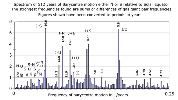

Going back to Timo Niroma’s ascii art plot of the distribution of solar cycle lengths, I note your chirp doesn’t have peaks around 10.38 and 12 years. But the Tomes z-axis FFT has 10.4 and 5.9=Ju/2
Here’s the Svalgaard power spectrum:

By The way, I’ve made this thread into a ‘sticky’ which stays at the top of the site, because it’s still going strong!
Hooray!
“David says:
March 7, 2011 at 7:08 am
The 7% TSI flux on an annual basis is very large. Does anyone have a SST chart which shows how SSTs lag this flux?”
The input variation for the whole earth is as shown but the earth axis is tilted so there is a north/south variation during the year.
Something else just occurred to me. The basic physics, which is played down in certain circles, is very simple: the body temperature follows square law versus orbital distance from the heat source, the sun.
I haven’t tried to calculate how large that is, ie. whether there ought to be a square law term. That needs doing as a cross check on whether the data is what it claims to be. (might be the distance variation is so small it is irrelevant)
Cold Sea Upwellings on the Costa del Sol, Spain
http://www.malaga-weather.com/article.712.html
Robert E. Phelan says:
February 21, 2011 at 1:14 am
Any significance to all of the waves trending down at once, as the graph shows them doing now?
Bond Event Zero….
Cross check clone of Leif’s result, yes it matches, we are talking the same thing.
Ignored <4 year, not useful. Longer periods should be taken as dubious given the very short data length and limitations of DFT.
Notable are two items: –
1. The spectral broadening of the 11y line. This means the region is confused/chaotic/modulated, whatever it is. (broadening is fairly literal language)
2. The just under 10 year line is sharp. This might be the second harmonic of the solar system dominant gravitational force @19.8 years.
Malaga View says:
March 7, 2011 at 2:43 pm
“Cold Sea Upwellings on the Costa del Sol, Spain…”
Good example of an unexpected micro event, thanks Malaga. I expect there are many other types of these sort of things which have slipped under the radar as being “small enough to ignore”. However, many small coincident events can have just as big an impact as one big one.
Perhaps no surprise climate science still doesn’t understand the way energy levels change in our oceans.
tallbloke says:
March 7, 2011 at 9:04 am
“By The way, I’ve made this thread into a ‘sticky’ which stays at the top of the site, because it’s still going strong!
Hooray!”
Hooray indeed! This thread has hit the 200’s partly due to my miss-post 2 above – sorry for that.
This thread seems to be getting to the nub about how the planetary orbital cycles effect the solar climate cycle, which in turn affects the climate on the planets. Many thanks to Tim, Tallbloke and contributors, without which it would not happen.
Thanks Tenuc for your contributions.
I really do think we’ve made some real progress here. Tim’s software is remarkable, and is helping to narrow down the important cyclic periods form an all too long list which previously stymied us with it’s myriad choices.
It will take time to reflect on what needs to be attended to and investigated further, but off the top of my tired head, the strong climatic signal whch coincie with important planetary periodicities seem to be those at around:
10.4 v
~11 Schwabe and JEV
12 ^
19.8 Jup-Sat
~45 Mars
55.15 JEV again
~80 Gleissberg
~110 Oceans
~220 De Vries
~440 (2x De Vries)
~2250 Jup and Uranus?
~4627 N+U+J+S
There is much to investigate in these cycles, plus the mysterious big ~35 year peak in Tim’s Chirp. 2x Ulric’s mysterious ~17 year solar wind cycle?
Ulric’s expostion on the 2225 year cycle sometimes involving an extra 179 year cycle is a hint that these relationships shift over longer timescales. The planets never repeat their orbital relationships twice. All ‘rules’ are contingent on a timescale, and new relationships will come to predominate over old ones eventually.
I suspect this is why the shift from ~40,000 year glacials to 100,000 glacials came about.
It should be noted that annual and monthly spectrum analysis of SSN gives slightly different results. L.S’s FFT power spectrum is for the monthly values, which I think is superior.
Quite so, the better resolution the better but this also hits a major problem in datasets, violation of Nyquist and Shannon, almost universal in climatic. This hurts if you do deep analysis. Don’t think it is appropriate to post details here.
The pair of plots I put up (few posts back in this thread) was deliberately one of each timeseries, identically processed and displayed. There is less difference than I expected.
With ssn the problems are compounded by inconsistent data gathering (including historically weather problems) and solar rotation.
I was hoping Leif was going to publish a fine time resolution corrected dataset.
Thanks for the reminder about Nyquist, Tim. Another reason why we need to be careful not to read too much into low sample rate/spacial resolution data. Nice video here showing aliasing…
There is also the question of how well a simple count of sunspot indicates solar activity. We know, for example, that the L&P effect appears to be reducing the number of visible spots and if the same thing has happened before how much should we trust sun spots as a proxy for the historic solar activity record?
Latest L&P chart here, courtesy of Leif Svalgaard…
This one is even more fun
Tenuc
Although the L&P effect has similar trend as shown in my formula
http://www.vukcevic.talktalk.net/LFC14a.htm (and in a way would back it up)
I am a bit suspicious of Svalgaard’s over-emphasising the effect (possibly to justify if his prediction is off the mark). It may be something popping up at the time of a deep minimum, but I am not convinced that it is a long lasting effect. http://www.vukcevic.talktalk.net/L&P1.htm
[…] back radiation, oce…tallbloke on tallbloke: back radiation, oce…vukcevic on Tallbloke and Tim Channon: A c…tallbloke on Dr David Hathaway: New lower s…tallbloke on tallbloke: back radiation, […]
tallbloke says:
March 7, 2011 at 7:15 pm
“..the mysterious big ~35 year peak in Tim’s..”
c. 13102 days = S/N synod.
With Mars, it depends what you include with it with. With J+E+V it`s on average a 44.75yr cycle. With just E+V, it`s 32yrs as a basic return, though this slips, and it moves from all 3 on one side, to E+V opposite Mars, and back to all 3 on one side, over a 299yr cycle.
c. 13102 days = S/N synod.
=35.87 years.
The ‘slipping and returning periodicities’ are interesting too.
Thanks Ulric
[…] the reconstruction of solar activity since 1610 made by NASA’s Judith Lean. This thread attracted a lot of interest, with over 200 responses in comments so far. Tim has also used the software he created to do cycles […]
[…] are homing in on the relevant periodicities. Along with the de vries cycle around 220 years and the ocean air […]
[…] Lanscheidt in 1988. Tim C and I came to the same conclusion last year, with our study on the cyclicities making up the solar variation. We published a plot giving a 50 year […]
[…] Tim Channon used his clever software to model the Steinhilber, Beer and 10Be TSI proxy back in early 2011 when we wrote the article on his reconstruction of Lean’s TSI. […]
[…] him out with a bit of Talkshop hindcasting and prediction skill here. Back in feb 2010 Tim C and I posted an article on replicating Judith Lean’s TSI reconstruction using the underlying sinusoidal oscillations […]
Tim / tim212 / tchannon,
regarding the sinusoid parameters you depicted above at February 26, 2011 at 8:48 pm.
When I make a bunch of sine formulae with those parameters and sum them I do not get anything like the Lean TSI reconstruction. Is there some special sauce missing?
The first couple of formulae are…
c1=$V$2 * SIN(2*PI() * ($A2-$W$4)/$T$2 – $U$2)
c2=$V$3 * SIN(2*PI()*($A2-$W$4)/$T$3 -$U$3)
…which in your terminology means…
c1= Amp1 * SIN(2*PI * (t-YOffset)/Period1 – Phase1)
c2= Amp2 * SIN(2*PI * (t-YOffset)/Period2 – Phase2)
c3..c17 are the same.
…and final amount…
TSI(t) = 1365.7 + c1 + c2 + (etc…)
In my implementation I’ve used the components with the 17 shortest periods as I figured the longest two made no difference over a 300 year test interval.
The YOffset is set = 0 but I thought there was a chance you might have measured time from something other than t0 = 1AD.
What’s wrong with my formula?
What formula can be used to approximate TSI from your cycle analysis?
Disjointed shorthand.
There are too many files to figure out which exactly, all in an earlier format, I was still developing the software, newer would read and translate, too busy on other things at the moment.
Easiest thing to do is grab an SBF data which looks sensible, not sure which version was used, take some guesses and point the software at it on auto. Upload the result as a working result
https://tallbloke.files.wordpress.com/2013/12/sbf-2009.zip
sheet 1, sbf data, added offset to AD time
sheet 2 live model (you might be able to work out the maths used from that, no I don’t type that fast :-), software writes the template for extending)
sheet 3 data for plot and plot if it survives into your software
Highest frequencies are not handled so it looks underwhelming.
I’ll email you, reply if you want to discuss… otherwise I will probably forget given so much else is going on.
Hey Tim,
Only just read your reply today.
Thanks for the spreadsheet, it was plug’n’play. It seems to get the gist of the TSI variation.
As you say, the high frequencies are absent, but that’s probably not irreparable… In the short term the TSI seems to modulate along with the sunspot count. Since I need short term TSI for short term projections I’m going to use (1365.4 + SSN/137) as an approximation of TSI for the time being.
For the longer term projections, perhaps some combination of RJ’s sunspot formula and these cyclic TSI components will work, but that’s for another day.
It’s good to be busy, eh!
Thank you everyone for this awesome presentation. I also am an audio engineer from way back when I made stereo amplifiers, and recently realized what the problem is with TSI measurements. They don’t measure everything because they can’t based on the frequency response curve of the measurement instruments. See http://www.ngdc.noaa.gov/stp/GOES/doc/GOES%20XRS%20readme.pdf and let me know what you think.
It appears the instrument can’t possibly respond to the full solar signal at all wavelengths.
Good find Bob, lower level information is sorely lacking.
The instrumentation is riddled with problems.
Good chance the transient response & SNR are inadequate too. Must fact check however.
Not sure transient is applicable as such, it’s a natural source with indeterminate rate, proably good enough provided they stick to Nyquist. All comes under good enough.
Noise is a different game, most of this stuff is at the limit.
If you look at the known solar UV and out towards gamma there is a pretty obvious noise floor problem… or is it, we simply don’t know.
A further problem is looking through a fog, and with magnetic fields present.
[…] https://tallbloke.wordpress.com/2011/02/21/tallbloke-and-tim-channon-a-cycles-analysis-approach-to-pr… […]
[…] https://tallbloke.wordpress.com/2011/02/21/tallbloke-and-tim-channon-a-cycles-analysis-approach-to-pr… […]
The top panel of Tim Channon’s model comparison with Lean’s 400 year TSI model contains a very interesting feature regarding the contentious issue about the slope differences between the ACRIM and PMOD satellite TSI composite time series during solar cycles 21 – 23. The agreement in periodicities between the Lean model and Tim Channon’s is amazingly good on most time scales, even those long compared to a solar cycle. The glaring exception to this is during the last two decades of the 20th century wherethe models diverge and Lean’s model shows no net trend while Channon’s model increases during 1980 – 2000. Channon’s model agrees with the upward ~ 0.04%/decade trending of the ACRIM satellite TSI composite. Lean’s model agrees with the Frohlich/Lean PMOD TSI composite. This result, along with other recent analyses (http://rd.springer.com/article/10.1007%2Fs10509-013-1775-9#page-1) provide further support for the ACRIM TSI composite’s upward trend and the probability that global warming during the late 20th century had a significant, if not dominant, solar forcing component.
Dikst: That’s a good observation, Thanks. The integration of sunspot numbers as a cumulative departing from the average over the period of record rises from 1934 to 2003. Although the peak amplitudes fell from the peak of cycle 19, the minima were brief, and the up/downramps steep, and the peaks sustained.