


Figure 1
The plot shows how the GHCN V2 station location has moved in time as a global average. Hadcrut3 is shown for illustrative purposes only (**).
I computed this some time ago and really needs someone else to carry out the same exercise in case I have made a significant mistake.
The software routine crawls around station data files extracted from the GHCN V2 distribution dataset. Some location data is missing, so at best this is an approximation.
In relation to datasets derived from this data there is little if any information on which stations are used and which ignored.
Bias
There is a well known bias east/west and north/south.
Correlating the direct results or the vector sum does suggest cause for concern. An upper limit might be for Latitude with an rsqr=0.41 but less for more recent times only. I am not a statistics expert so welcome any insight from that point of view. I can probably make the computed result available
Expect a further related post on GHCN and derived series. All part of showing works here which would otherwise be lost.
[edit] There is a wealth of dataset information in XLS ’97 Spreadsheet format here, 5.2M. I have put many datasets into sqlite and but this is an extract of basic information for GHCN V1, GHCN V2, MetOffice 10, Jones from disk files. There are likely to be mistakes given the state of some of the data plus I am human. Some were identified as former “missing” station sets by Warwick Hughes who has been involved with the data saga for many years, information on this can be gleaned from his web site http://www.warwickhughes.com/blog/ Warning, this does not tell you about the fragmentation within a time span, an important factor.
[/edit]
** Hadcrut3 is compiled from CRUTEM3 and HADSST2. It is Crutem which is directly based on the GHCN data. I don’t have the equivalent official time series to hand and is little different from Hadcrut3.
Tim (not Tallbloke)

Hi Tim:
Interesting way of presenting the data. I’ll take a look at the stations I use tomorrow to see how they compare.
“There is a well known bias east/west and north/south”. What’s the basis for this claim?
Average location. Interesting concept. Translates to bias in choice of stations sampled, I assume?
Roger, I’ve read that various places, no reference. As land based there will be more northern stations. Early on the US tended to dominate, then slide back more towards Asia.
Brian, ideally the mean of station location should be fixed over time and on zero, zero, middle of the signed lat/long, the central reference.
I expect there are better and different ways of representing the concept. Prefer simple.
Lapse rate is something I am peripherally interested in at the moment but that story is long and incomplete.
I have a suspicion that silent station changes (not documented) have led to significant errors but there are only a handful of definite instances, such as move to airport which is at a slightly different altitude. See why I wanted pressure data. For the moment I will leave that one for investigation later.
Tim – Thank you – wonderful analysis.
If you have the time or inclination it would be great to see additional details from your analysis:
1) Station Count by Year
Counting the number of stations per year would be very interesting, especially if you could separately track the number of stations added and dropped in each year. To pick up on the East-West and North-South divides it would great to see the station count tracked individually for these four points of the compass.
2) Average Altitude
To pick up on the East-West and North-South divides it would great to see the average altitude tracked individually for these four points of the compass.
3) Average Longitude
To pick up on the East-West divide it would great to see the average longitude tracked individually for these two points of the compass.
4) Average Latitude
To pick up on the North-South divide it would great to see the average latitude tracked individually for these two points of the compass.
This is all because the manmade volatility in the station data tells a very interesting story… a story in Three Acts that reflects the settled science.
ACT 1 – 1992 – Stage Setting
The initial data set trawls the historic archives to establish the foundation. This was not a simple exercise. The data was carefully onboarded from the historic archive to establish the required 30 year based line. Starting in 1960 the volatility in the latitude, longitude and altitude of the station data suddenly levels off as the required base line is established.
ACT 2 – 1997 – Cosmetic Surgery
As the 1990s progressed it became apparent that the patient required urgent surgery. Thus, the surgeons knife removed some cold northerly carbuncles and the average longitude suddenly moves south by 10 degrees in the early 1990s. The surgeons knife additional removed some prominent cold warts and the average altitude suddenly drops by about 30 metres. However, the volatility of the metrics indicate that the patient’s medication has required continual fine tuning.
ACT 3 – 2011 – More Surgery
In 2011 the patient underwent more surgery… however, at this stage it is unclear whether more warts and carbuncles have been removed or other ailments have been addressed.
m-view;
Yes, the 1990 Great Dying of the Thermometers shows up quite clearly, doesn’t it?
To quote a famous German philosopher, Sgt. Manfred(?): “Very interesting. But stupid!”
😡
Tim:
I think the “biases” you refer to are related to NH/SH temperature trend differences. The NH consistently warms or cools faster than the SH (the NH warmed faster than the SH between 1910 and 1940, cooled faster than the SH between 1940 and 1970 and has warmed (much) faster than the SH since 1970) and there are a lot more stations in the NH. So if you take the arithmetic mean of all stations you will get a global series that’s biased towards the NH. The way it’s normally done, however, is to take the average of the NH and SH series, which generally gets around this difficulty, although it’s not a perfect solution. (One problem is that there aren’t enough stations in the SH to estimate reliable annual means before about 1920, meaning that we don’t have enough data to estimate a reliable global mean before about 1920.)
A more robust way of doing it is to area-weight the results inside smaller latitude bands (75-90N, 60-75N etc,) but it doesn’t make much difference when you do this.
The proper way of doing it, and the way I do it, is to segregate the data into areas where all the stations show substantially the same temperature trends – but trends which are significantly different to those in the surrounding areas – and area-weight the averages. This gives about the same results too.
However, the temperature trends in the 64 areas I’ve identified vary enormously, so if anyone wants to claim that there’s really no such thing as a “global” temperature time series I’m not going to argue with them. 🙂
I don’t think “longitude bias” is an issue, and minor changes in mean station elevation shouldn’t be one either if temperatures are expressed as anomalies relative to a 1950-80 (or whatever) baseline.
Tim
You say: “I have a suspicion that silent station changes (not documented) have led to significant errors”
If you assume that station changes introduce distortions that are random in sense and magnitude, which all the evidence I’ve seen suggests they are, and if you assume that station changes occur on average once every 20 or 25 years, which they do in the USA, then you don’t have to average many records together before the errors begin to cancel out. Besides, records that are seriously distorted by station changes are usually easy to identify and weed out.
The problems occur when people start trying to “correct” for these changes.
The USHCN “corrections” to the US temperature records, which were designed to correct for stair-step shifts introduced by station changes, are an example. I believe they’ve been modified since I reviewed them ten years ago, but here’s a brief summary of what I found at the time.
* About half of the corrections matched identifiable shifts in the raw record. The other half introduced artificial shifts that weren’t there to begin with.
* The corrections were evenly split between warming and cooling. However, the average cooling correction was 0.3C while the average warming correction was 0.4C.
* Records that showed warming didn’t receive net warming corrections. Records that didn’t show warming did.
* Net result: The “corrected” US records showed about 0.3C more warming than the raw US records.
* And 1998 replaced 1936 as the warmest year on record (which I think was the purpose of the exercise)
And then GISS went ahead and overwrote over 1,000 raw US records with the USHCN “corrected” records in its GISTEMP data base. (Shame on you, GISS.)
You might also take a look at the Australian records, which courtesy of the Australian Bureau of Meteorology suffered the same fate as the US records at about the same time. And now that I think of it, the New Zealand records did too.
As I mentioned earlier, the problem isn’t the raw records, it’s the “corrections” that get applied to them.
@Roger and Tim: This has been heavily covered by E.M.Smith on his blog, see ,
Many valuable graphs and observations of his own and from commentators. pg
I hadn’t seen Mr Smith’s posts.
The basis is more about GISS and the US, not read it in detail.
For the time being I am looking at the software, written some time ago and I want to make some changes. If I do I will probably update figure 1 and then as a new post deal with the counts, which is actually the real end goal of all the GHCN posts, there is a twist.
Sorry if I seem to be ignoring people, didn’t sleep last night, best if I do limbo.
I’ve updated the post by adding a link to a large spreadsheet about the contents of various station datasets. Just tables of names and figures, thousands of rows.
Tim: Good work with the spreadsheet. I can use it. Thanks. 🙂
tchannon says:
November 10, 2011 at 12:45 am
I’ve updated the post by adding a link to a large spreadsheet about the contents of various station datasets. Just tables of names and figures, thousands of rows.
Thanks Tim…
I have been taking a look at the GHCN Start Date and End Date columns in your spreadsheet.
1) The Version One data looks fairly impressive at first sight:

6,039 stations covering 1701 through to 1990
2) However when you zoom into the period starting 1900 things get interesting.

Evidently lots of new stations came online in 1931, 1941, 1951 and 1961.
Perhaps these were used to set the narrative for each decade!
3) The Version Two data looks even more impressive at first sight:

13,471 stations covering 1701 through to 2009
4) However when you zoom into the period starting 1900 things get interesting.

a) The are still lots of new decade narrative stations for 1931, 1941, 1951 and 1961
plus lots of new fiddling for 1948 and 1949… not sure why… perhaps it was the move to the airports.
b) The Great Dying of the Thermometers during the 1990s is very evident.
c) But the really new thing for me is the new bubble of stations that starts in 1986.
It looks like a whole new set of Global Warming stations were introduced to the narrative.
5) The overlay of V1 and V2 data shows how much they have had to change the story to keep the narrative alive.

Was hoping that would enable a good take by someone else. It has.
Note: what you _cannot_ see is broken datasets where eg. 1900-1910 and 1980-2000, things are worse.
It would take me days to present that in a usable form, invent and write the code, figure out how to pass the data across.
There is more, oh yes, 🙂
There is more, oh yes, 🙂
The number of years (duration) for each station make interesting reading…
The data forms a layer cake where decade has been filleted and spiced up.
Historically a station was only incorporated if it had at least 10 years worth of data…

But their final cherry on the cake is a desperate hack of short station data…
Short station data tohide the decline since 1960?
Short station data tomake the incline since 1960?
Recipe for the GHCN V2 Layer Cake
Step 1 – Dice and Slice
Lay out on the slab the base Version One data mixture.
a) Peel off a superficially thin layer of historic station data and save for later use.
b) Cut off a base layer of stations starting prior to 1900.
c) Cut the remaining stations (starting after 1901) into 10 decadal slices.
Step 2 – Layering the Cake
Now start building up from the bottom the layer cake.
Take each slice in turn and perform the following layer processing
d) Make the layer manageable by filleting out offending / lumpy / distasteful stations.
e) Add new season stations at the start of the slice for added jest and spice.
f) Fine tune each year of the slice for texture and richness
g) Review the accumulating stack of slices for flavour and smoothness.
Step 3 – Cake Decoration
h) Ice the cake with the thin layer of historic station saved from Step 1a).
i) Chop some new stations data from after 1960 to make a hot cherry for the top of your cake.
The GHCN V2 Layer Cake – Sliced by Altitude

There is very little station data to analyse…
But what this is shows the stations have moved to lower (warmer) climes.
The GHCN V2 Layer Cake – Sliced by Latitude

There is very little station data to analyse…
But what this is shows the stations have moved to lower (warmer) climes.
MV and Tim:
I’ve been reading your comments with interest, but the basic question is whether all the GHCN station changes you’ve identified have biased the surface air temperature record. I ran some checks on this and here are the results.
I started with the GISS “meteorological station only” global surface temperature time series, which is constructed using over 6,000 surface station records from the GHCN data set.
I first compared the GISS series with the global series I had constructed from my own data set, which contains 900 selected and unadjusted surface station records that I am fairly confident are free of UHI impacts and other distortions. The two series weren’t identical, but they were very close even though GISS used over 5,000 more records than I did.
Having discarded over 5,000 station records I then proceeded to discard some more. From my data set I selected the 128 stations that had continuous records between 1950 and 2005 and discarded the 772 that didn’t. Then I reconstructed the global series between 1950 and 2005 using only the 128 records and compared it with GISS. The two series still matched very closely and both showed the same warming gradient over the 1950-2005 period (0.13C/decade)
Then I threw out some more stations. I sorted the 128 stations by latitude, discarded every other one and reconstructed the global series using the remaining 64 stations. This series still compared quite well with GISS and the 1950-2005 warming gradient remained at 0.13C/decade.
Then I threw out every other one of the 64 stations and reconstructed the global series using only 32. The match with GISS became a little more ragged, but the 32-station series again showed a 1950-2005 warming gradient of 0.13C/decade.
So here are five different global surface temperature time series, one that uses over 6,000 GHCN stations, one that uses 900, one that uses 128, one that uses 64 and one that uses only 32, and they all show the same amount of warming since 1950. This of course doesn’t prove that the series are correct, but I think it does show that changes with time in GHCN station locations, elevations, instrumentation etc. haven’t had a significant impact on warming estimates, at least not on the global scale.
Roger Andrews says: November 18, 2011 at 7:53 pm
So here are five different global surface temperature time series, one that uses over 6,000 GHCN stations, one that uses 900, one that uses 128, one that uses 64 and one that uses only 32, and they all show the same amount of warming since 1950.
Combinations of 6000, 900, 128, 64 and 32 stations all show the same amount of warming since 1950.
Same signal at across all the global… no differences by urban / rural / altitude / latitude / region…
Amazing!
Do you really expect anyone / everyone to believe that this result reflects the REAL WORLD?
The same signal across all the globe.. across all the climate regions… across all stations….
Can’t they just cut down GHCN to just 16 or 8 or 4 or 2 or even 1 station?… the technique has been proved using station data from Russia… with a few stations they might actually be able to calculate a real Daily Average Temperature from data logged every hour… or even every minute… Not the Daily Extremes Mid-point [based upon (Tmax + Tmin) / 2] nonsense they currently produce…. perhaps we could then discover how this same amount of warming since 1950 is occurring – such as: New high HIGH temperatures, more high HIGH temperatures, new high LOW temperatures, more high LOW temperatures, etc.
PS: They are actively working on reducing the number of stations… in 2009 there were just 1,596 stations left… very close to the 1,538 stations reporting in 1890.
That is what I call remarkable progress 🙂
Okay, starting to lift the lid, I posted originally with good reason. Not decided yet on what to show or how much.
Here is a crazy one. Hadcrut3 is derived from stations in GHCN V2 via CRUTEM3 and HADSST2
A quick plot of a very unusual kind, to do with phase. The bizarre thing is the right hand end, straight line all of a sudden, then I twigged this is the satellite period.
Not sure whether to simply put this stuff in this thread or as a full post. A lot might be coming.
tchannon says: November 19, 2011 at 4:13 am
A lot might be coming.
It deserves a full posting / airing.
Hadcrut3 is derived from stations in GHCN V2 via CRUTEM3 and HADSST2
Personally very intrigued by the overlaps / similarities / incestuous relationships between the main Team Series.
Especially: how do they manage to produce numbers that are always in the same ball park?
Ground station data above 70 degrees north is very sparse.
Ground station data above 50 degrees south is very sparse.
Ground stations are of varying quality and accuracy.
Ground stations are not uniformly distributed.
Ground station selection varies [filleted, chopped and diced] over time.
Ground station averages are based upon (Tmax + Tmin) / 2.
Ground station data is then adjusted in the computer blender.
Ground station data is then gridded and infilled.
Satellites scan strips of the globe as they orbit.
Satellites scan strips have multiple overlaps at the poles.
Satellites scan strips have gaps – generally at mid-latitudes
Satellites scan strips don’t always scan exactly the same strips.
Satellites scan strips randomly capture the daily HIGH for any location.
Satellites scan strips randomly capture the daily LOW for any location.
Satellites scan strips are generated from multiple angled sensors.
Satellites scan sensors have to “interpret” differing areas / surfaces / clouds / dusts / weather etc
Satellites scan strips use different algorithms to interpret each angled sensor.
Satellites scan strip sensors are not calibrated against temperature readings on Earth.
Satellites scan strips must be untangled (with overlaps deduplicated) during monthly processing.
Satellites scan strips must be merged into standard strips during monthly processing.
Satellites scan strips must be time synchronised and averaged during monthly processing.
Satellites scan gaps must be ignored or infilled during monthly processing.
Satellites scan data cannot be independently inspected, reprocessed or reconciled.
Given the above set of challenges I am left with the following taboo question:
HOW can ground stations and the Satellites produce numbers that are in the same ball park?.
This questions is particularly aimed at IT specialists, statisticians and auditors 🙂
There are lots of possibilities:… but none of them reflect the real world raw data.
Some details regarding the satellite technical challanges…
Note: Bold, italics and [bracketed comments] are mine.
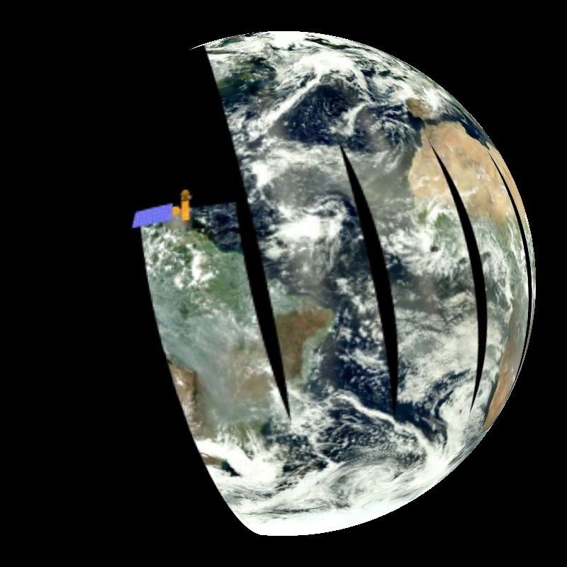
Aqua Satellite and MODIS Swath
And Wikipedia regarding UAH…
Perhaps the most important common demoninator is: gridding.
MV
“Combinations of 6000, 900, 128, 64 and 32 stations all show the same amount of warming since 1950. Same signal at across all the global… no differences by urban / rural / altitude / latitude / region…Amazing! ….Do you really expect anyone / everyone to believe that this result reflects the REAL WORLD? The same signal across all the globe.. across all the climate regions… across all stations….”
No I don’t, because that isn’t what I said, as you would know if you had read what I said.
But let me reply in a constructive manner anyway.
I performed the same sort of analysis as you and Tim C are now doing ten or more years ago, and starting with the same assumption – that the surface air temperature series was wrong. I was in fact so convinced that I could prove this that I spent two years, on and off, sorting through thousands of raw GHCN records, accepting those that were verifiable, rejecting those that weren’t and throwing out any that showed obvious UHI impacts. Then I reduced the records I’d selected to a common baseline and segregated them into 64 different “climate regions” where temperature trends were the same but significantly different to those in the adjacent regions, which was a much more robust approach than the grid-square averaging method in use at the time. Finally I area-weighted the regional means into hemispheric series, took the mean of the hemispheric series to get a global series, plotted it up –
– and found that it matched the GISS “meteorological station only” surface air temperature series almost exactly.
Must have done something wrong, I thought. So I went back and started adding stations, subtracting stations, using different averaging procedures (latitude-weighting, simple arithmetic means, first-difference etc.) but no matter what I did my series still matched GISS.
As a result of this failed effort I am now convinced that the global surface air temperature record is correct relative to the data used to construct it. If you want to check me out on this you can try constructing some series of your own, but I can pretty much guarantee that you will get the same results as I did.
As I stated in my previous comment, however, this doesn’t prove that the surface air temperature series is right. It’s intriguing to note that over the period of satellite record there’s a close global match between SSTs and UAH lower troposphere temperatures, with the SSTs showing 0.43C of warming between 1979 and 2010 and UAH showing 0.45C, but not with surface air temperatures, which show 0.63C of warming over this period. Is this difference a real climatic effect or are the surface air temperature records warming-biased? Don’t know for sure, but if there is a warming bias in the air temperature records it’s caused by something other than UHI impacts or station changes.
Tim C:
“Here is a crazy one. Hadcrut3 is derived from stations in GHCN V2 via CRUTEM3 and HADSST2”
I’m not sure where the craziness comes in, but HadCRUT3 – the world’s “official” surface temperature time series – is indeed an area-weighted average of HadSST2, which is an SST “ocean” series, and CRUTEM3, which is an air temperature “land” series with SSTs used to fill in some of the blanks. Leaving aside the question of whether it’s valid to mix SSTs and air temperatures (it isn’t), the point is that HadCRUT3 is about 70% based on HadSST2 and only about 30% based on CRUTEM3, which means that errors in HadSST2 will have over twice the impact of errors in CRUTEM3. So if you’re looking for skeletons in the Team’s closet you should focus your attention on the SST record, not the surface air temperature record.
And if you do this you will find that HadSST2 is not just wrong, but seriously wrong. I went into the question of why in a post over a year ago, and I’m reposting a link to my analysis below. I hope you can find the time to read it . 🙂
Click to access final-sst.pdf
Lot of work in there.
Keep an eye on email.
Listen up!
Look in the comments here, is SST stuff right now
The post at CA includes this plot of 2nd time differential of temp. It highlights both the early war drop and the post war spike. Post war SST shows that warming “acceleration” continues to be present until about 1980 in diminishing proportions. That is not at all evident to the eye when looking at the time-series of temperatures. I’m not sure whether the net bias is + , – or net zero. Be careful not to jump to conclusions by eye.
It also shows that both Berkeley and Crutem3 (esp. B-est) show anomalous negative accel around 1990. Jeff Sherriden suggests this maybe problems with T-obs, which seems likely. It also ties in with the great dying of thermometers that this thread highlights.
[ thank you for taking the time and effort to post here: Tim]
BTW I have also posted scripts on that thread on CA to do the diffs, the gaussian filtering and reproduce the graphic.
TB, you may like to look at using gaussian instead of running mean when looking for cause and effect. RM can cause some unexpected effects (to those who don’t find out the characteristics of a filter before using it) , these include letting though significant amounts of stop band frequencies, ie bad smoothing, bending peaks left and right, truncating and even inverting peaks depending on what is happing either side.
here’s the frequency response of the two:
[copy of linked image placed on WordPress servers and shown here, original {http://tinypic.com/r/nevxon/5 : Tim]
These effects can lead to false attribution or reduced correlation where there is a real effect.
Looking again at this plot with reference to the Follands’ folly question:
There is a downward trend in 2nd diff that appears possibly abnormal in the context of the cyclic pattern that was established before the war. However, I do not see the sort of step change that would be in clear evidence if this EIR adjustment was totally wrong.
If it was applied too abruptly there should be massive negative in d2T/dt2. There is not.
On the other hand, there is a very sharp uptake just after the war that definitely does look suspect. The fact that this is not reflected , in the slightest, in the land record data suggests strongly that it is anomalous. It is hard to see show such an abrupt change in SST could occur without it being very evident in the land temp record.
My conclusion would be that it is the whole period 1938-52[*} looks to have serious issues but the upswing looks more anomalous than the preceding downward trend.
I would encourage more examination of the time derivatives in researching this kind of issue, since it would take either a very skilful fraud or a very skilful correction to not show some discontinuities in T(t), dT/dt and d2T/dt2.
[* correction}
correction : 1938-52
My conclusion
would be that itis the whole period1930-52looks to have serious issuesbut the upswing looks more anomalous than the preceding downward trend.>>
Brian, ideally the mean of station location should be fixed over time and on zero, zero, middle of the signed lat/long, the central reference.
>>
And if the arbitrary point of reference was centred on Beijing instead of London where would you expect the idea mean station position to lie?
Tim , I suggest you grab the scripts I put up on CA and run the results up on gnuplot in interactive mode. You can then zoom in to examine any period of interest in monthly resolution if you wish.
That will help you see if there are any anomalous changes associated with the steps and trends you have highlighted with your initial plot here.
P. Solar
Over at CA you say: “I have found what looks like clear proof of Jones’ “cooling buckets” adjustment being grossly over done …”
It’s nice to know that I’m not the only one crying foul.
But I don’t think we don’t have to go to second vertical derivatives to show that the bucket bias shift adjustment is bogus because it’s obvious in the unmodified time series. I discuss this in detail in https://tallbloke.files.wordpress.com/2011/02/final-sst.pdf.
The important consideration, however, is what happens when this bogus shift adjustment is removed. Here’s a brief summary:
1. It becomes obvious that SST and SAT trends are different, at least on the multidecadal scale. The historic assumption that they should be the same over all time scales, which was the basis for applying the shift adjustment in the first place, is invalidated.
.
2. If SST and SAT trends are different we must treat them separately, in the same way as we treat the SAT and UAH troposphere series separately. We don’t get meaningful results when we combine SST “ocean” series and SAT “land” series into an apples-and-oranges “surface temperature” series.
3. And if we don’t get meaningful results by combining SSTs and SATs we have to junk HadCRUT3, which does just that. (With the shift adjustment included it’s wrong anyway.)
4. We also have to junk HadSST2, which because of the adjustment underestimates total SST warming by +/-0.5C. (Although paradoxically this doesn’t reinforce the case for AGW. It actually reinforces the case for a solar influence on climate.)
Enough to be going on with, I think.
The server at jisao.washington.edu is taking too long to respond.
Is that URL for the ICOADS data in ref 1 still valid?
Responding PDQ from a good UK connection, too fast, so I guess it has recently been reset.
I think that paper brings up an important issue. I was not aware of this one sided adjustment. But I don’t see the use of being inexact when taking others to task for being inexact.
>>
It shifts the entire ICOADS SST series after 1942 down by almost 0.5C relative to the series before 1940.
…
If a bucket-intake change indeed caused a permanent 0.5C upward shift in the SST record after WWII then intakes must be biased at least 0.5C high relative to buckets, but the 0.7C Saur estimate at the top of the Table is the only one that exceeds this threshold. Most of the later estimates are in the 0.2-0.4C range, enough to explain only about half of the shift.
>>
You don’t seem to have done any mathematical assessment so you appear to reading off by eye. Doing the same I’d say the drop is between 0.4 and 0.5 , it’s certainly less than 0.5 and then diminishes in time to be about 0.25 C.
So “almost 0.5” is “about twice” the lower end of that bracket.
You could also say almost 0.4 is about *equal* to one time the upper limit and hence the magnitude is about right.
I think you could be more objective on that.
It seems from the other papers you refer to that 0.3C is a likely value, This would match the long term difference in the two versions seen by y2k. So the 2/3 bias globally would be close to 0.2C (by no means insignificant in relation to estimated warming).
The HUGE defect in all this is that the adjustment was applied (progressively) over a very short period from 39-42 but not removed after the war when that level of correction was no longer legit.
It seems something like 0.45 needs to be removed over the war years *only* , then 0.3 applied slowly over the following decades.
However, this does explain the anomalous dip after the war that has been bugging me since I started looking at all this.
It’s absolutely astounding that after the literally billions that have gone into modelling and climate research in general over the last 20 years, that they still have this sort of glaring error addressed in the very data against which they are calibrating their models.
P. Solar
“You don’t seem to have done any mathematical assessment so you appear to reading off by eye. Doing the same I’d say the drop is between 0.4 and 0.5 , it’s certainly less than 0.5 and then diminishes in time to be about 0.25 C.”
How do you come up with 0.25C?
“It seems something like 0.45 needs to be removed over the war years *only* , then 0.3 applied slowly over the following decades.”
Remove 0.45C over the war years by all means, but why add 0.3C back in over the following decades?
“It’s absolutely astounding that after the literally billions that have gone into modelling and climate research in general over the last 20 years, that they still have this sort of glaring error addressed in the very data against which they are calibrating their models.”
Actually it’s over the last 27 – almost 28 – years. The glaring error has been around since Folland, Parker and Kates first applied a permanent shift adjustment to the SST data in 1984.
And thanks for the reminder. I should have included this as point 5 in my previous comment. HadCRUT3 is not of the quality necessary to be used to calibrate/validate climate models, to put it charitably.
More later, probably.
Getting back to the subject of this thread, anyone who wants an example of how changes in station location, density, reading methods etc. can bias a data set should look at the SST data between 1938 and 1946.
P Solar, on rereading the CA thread Steve says
“Steve- interesting graphic. All hadSST is post-bucket adjustment. I’ve down estimates in the past of the amount but they are just estimates. You should place your code and results online so that people can look at your calculation easily.”
I didn’t notice other wise I would have replied *gridded* hadsst2 does not have bucket adjustment which seems to be a post processing step.
From a month ago
It’s not the difference but the differential : dy/dx , it is logged at the halfway point in the x interval so as to not introduce a shift. With the monthly data the 2nd diffs get pretty noisy which is why I ran a gaussian filter on them .
Sometimes a feature may stand out in the diff that is not obvious in the time-series (or vice versa). I first did this on the Berkeley data and it showed up what looks like anonymous adjustments around 1990.
In the case of the war time shift discussed here it helps to assess whether the impact of up swing is more/less/equal to the later down swing. It seems on the long scale it may be better to accept the ICOADS anomaly rather than Folland’s folly.
Another interesting thing to come out of examining the derivatives is the magnitudes. It is expected that land temps will be more volatile than SST but the difference between Crut and Berk is notable.
To get them to overlay reasonably closely I need a different scaling factor. One may suppose that Berk is more “sensitive” or Crut is smoothing changes out a bit in time, neither would be necessarily better or more accurate.
However, the same scaling applies to the long term trend. Berk recent warming is significantly stronger , by the same factor.
I don’t know what that means or why it is the case at this stage but this result will be very important for any inference about the extent of AGW.
This from FOIA 2011:
date: Wed, 23 Apr 2008 07:59:26 +0100 (BST)
from: P.Jones
subject: Re: CRU TS 3.0
to: t.osborn
Tim,
Thanks again for all your efforts. Maybe you’ll be able to write
the paper as well! I did start 9 months ago, so have a few
pages.
I always thought this ought to have been much easier than
it seems to have been. Very good that Douglas will do the
DTR/Cloud work if you can get the support.
I just wish that Harry had more of a feel for what he’s been
doing. I should have gotten Harry to produce more results as
he was doing the original work. I assumed he’d gotten things right,
as I thought it was just a matter of getting Tim M’s programs to work.
He ought to have looked at the fortran rather than Tim M’s comment
lines.
Cheers
Phil
> Hi Harry,
>
> thanks for the email re. the VAP data. Yes, go ahead and delete those 3
> stations and recreate. That should, I hope, solve the main problems…
> and more minor problems can wait for some future time when we actually
> have time to worry about more minor things!
>
> Regarding the extensive and strange banding problems found in the new
> variable (wetdays), I think I may have found the cause. As I mentioned
> earlier, it is the synthetic wetdays that have the banding in them.
>
> Looking at the rd0_gts program in
>
> /cru/cruts/version_3_0/BADC_AREA/programs/idl/rd0_gts_tdm.pro
>
> which is what you used to produce the synthetic wetdays, it seems to be
> reading (see lines 19 and 22) gridded normals for precipitation and for
> wetdays from files
>
> ../norms_05_binary/glo.pre.norm
>
> and
>
> ../norms_05_binary/glo.rd0.norm
>
> Now, from the directory name (the ’05’) and from the code (the 720*360 on
> lines 18 and 21) and from the size of the files it’s reading, my guess is
> that these are normals on a 0.5 degree grid. But the precip anomalies
> that you’re reading (from ../prebin/) are on a 2.5 degree grid (following
> Tim M.’s instructions for synthetic data), and the output it produces is
> on a 2.5 degree grid.
>
> What will happen, therefore, is that when rd0_gts attempts to extract pre
> and wet (rd0) normals for all the 2.5-degree land boxes from the
> 0.5-degree arrays of normals, it will pick up chunks of data from just the
> first 1/25th part of the arrays, sometimes picking up bands of land with
> non-missing values, and sometimes picking up bands of ocean with missing
> values. That would explain the banding.
>
> The solution seems to be to alter this program to read normals on the 2.5
> degree grid, assuming you have these. Presumably you do, in
> ../norms_25_binary/
>
> There may be a similar problem with frost days, since frs_gts_tdm.pro
> seems to be reading frostday normals from ../norm_05_binary/ too. However
> I haven’t checked the frostday data you have made, since I don’t need that
> variable — please don’t redo frostdays (at least until you have redone
> vap and wetdays), I’m just noting that the current file is likely to be
> wrong and hence not suitable for distribution.
>
> It looks like you already read 2.5 degree normals when making synthetic
> vap, which is why that doesn’t show this problem.
>
> The other thing to note is that the final output from rd0_gts is
> fractional anomalies * 100 — i.e. (wet-wetnorm)/wetnorm) — or you could
> call them percentage anomalies. I’m not sure, therefore, what you need to
> set synthfac to when you read these synthetic anomalies… maybe
> synthfac=100 rather than synthfac=10? It depends what units
> quick_interp_tdm2 wants to be working in. If it wants to work in
> percentage anomalies, then synthfac=1 (or omit synthfac) instead of 100.
> Presumably it needs the synthetic and actual wetday anomalies to be in the
> same units… looking at anomdtb.f90 (which I presume is how you made the
> actual station wetday anomalies) it seems (lines 490 or 504) to be
> multiplying fractional anomalies by 1000, which would result in percentage
> anomalies * 10! Not sure if this is actually what is happening since this
> is the first time I’ve looked at anomdtb.f90 and it seems fairly
> complicated! But it implies synthfac=0.1 might be needed! I guess we may
> need to use trial and error to find the right value for synthfac. I’d
> start with synthfac=100 since I think the values showed too little
> variability with synthfac=10 — however this may all change when the
> banding problem is solved!
>
> Basically… good luck!
>
> Cheers
>
> Tim
>
>
>
>
Here is if ICOADS with a simple 0.24C reduction during the period where there is the wartime shift.
There is no fade in/ fade out. Just look at the date, it’s a step change on both ends. I (arbitrarily) chose the initial step rather than the end step as the value to subtract.
The resulting record flows very naturally with the surrounding data before and after the war. Why anyone would device any more complicated way of doing this is beyond me.
There’s a dozen reasons why the war-time record could be different that are far more compelling that buckets. Any buckets and intakes argument needs to look at post war and to be justified on changes to the peacetime commercial shipping records not war-time blips.
The Hadley Centre’s (approx 0.45C) adjustment and way is was slowly blended in so as to make it a less obvious hack seems very unscientific and unprofessional, to be polite about it.
If their step was 0.25 and not 0.45 they would not have needed to blend it in the first place, this all smacks of “hide the decline” tactics.
The fact that they then totally ignored the corresponding post war drop is inexcusable. At that point it becomes blatant manipulation.
#5179
cc: Mike Wallace , Phil Jones
date: Fri, 16 May 2008 13:42:24 +0100
from: John Kennedy
subject: Re: Press release
to: David Thompson
All,
I’ve attached the latest version of the press release. I’ve stripped off
the additional information and removed some of the text about keying in
new data.
The press office and other interested parties haven’t seen it yet, which
is the next stage.
John
On Wed,REDACTEDat 10:50 +0100, David Thompson wrote:
>
>
> All,
>
>
> I’ve made a few tweaks to Mike’s version. Text is below.
>
>
> I was also uncomfortable with the Hadley Centre propaganda. I think it
> would have been a lightning rod for the critics.
>
>
> -Dave
>
>
> Using a novel technique to remove the effects of temporary
> fluctuations in global temperature due to El Niño and transient
> weather patterns, researchers at Colorado State University, the
> University of Washington, the UK Met Office and the University of East
> Anglia have highlighted a number of sudden drops in global
> temperature.
>
>
> Most of these drops coincide with the eruptions of large tropical
> volcanoes and are evident in temperatures measured over both the
> world’s land and ocean areas. But the largest drop, occurring towards
> the end of 1945, is unrelated to any known volcanic eruption and is
> not apparent over land. It appears to arise from an artificial and
> temporary cooling caused by an abrupt change in the mix of US and UK
> ships reporting temperatures at the end of the Second World War.
>
>
> The majority of sea temperature measurements available in
> international data bases between 1941 and 1945 are from US ships. The
> crews of US ships measured the temperature of the water before it was
> used to cool the ships engine. Because of warmth coming from the ship,
> the water was often a little warmer than the true sea temperature. At
> the end of 1945 the number of US observations in the data base dropped
> rapidly while the number of UK observations increased. UK ships
> measured the temperature of water samples collected using special
> buckets. Wind blowing past the buckets as they were hauled onto the
> deck often caused these measurements to be cooler than the actual sea
> temperature. The sudden drop in global-mean temperatures at the end of
> World War 2 is due to the sudden but uncorrected change from US engine
> room measurements – which are biased warm – to UK measurements – which
> are biased cool.
>
>
> Although the drop in 1945 is large in climate-change terms
#5198 mann to Jones cc Schmidt
Potentially the key issue is the final Nature sentence which alludes to the
probable
underestimation of SSTs in the last few years. Drifters now measuring SSTs dominate
by over 2 to 1 cf ships. Drifters likely measure SSTs about 0.1 to 0.2 deg C cooler
than ships, so we could be underestimating SSTs and hence global T. I hope Dick
will discuss this more. It also means that the 1961-90 average SST that people use
to force/couple with models is slightly too warm. Ship-based SSTs are in decline – lots
of issues related to the shipping companies wanting the locations of the ships
kept secret, also some minor issues of piracy as well. You might want to talk to Scott
Woodruff
more about this.
REDACTEDA bit of background. Loads more UK WW2 logs have been digitized and these will
be going or have gone into ICOADS. These logs cover the WW2 years as well
as the late 1940s up to about 1950. It seems that all of these require bucket
corrections.
My guess will be that the period from 1945-49 will get raised by up to 0.3 deg C for
the
SSTs, so about 0.2 for the combined. In digitizing they have concentrated on the
South Atlantic/Indian Ocean log books.
[2] http://brohan.org/hadobs/digitised_obs/docs/ and click on SST to see some
comparisons.
The periods mentioned here don’t seem quite right as more later 1940s logs have also
been
digitized. There are more log books to digitize for WW2 – they have done about half of
those
not already done.
If anyone wonders where all the RN ships came from, many of those in the S.
Atlantic/indian
oceans were originally US ships. The UK got these through the Churchill/Roosevelt deal
in 1939/40.
Occasionally some ships needed repairs and the UK didn’t have the major parts, so
this will explain the voyages of a few south of OZ and NZ across the Pacific to Seattle
and then back into the fray.
ICOADS are looking into a project to adjust/correct all their log books.
TB:
Have you ever wondered where some of these SST adjustments come from? Here’s how Folland and Parker 1995 came up with theirs (and FP is the “landmark” paper).
FP’s set out to correct the SST record for an artificial cooling bias caused by a supposed transition from insulated wooden buckets to uninsulated canvas buckets between the middle of the 19th century and about 1940. (There was some anecdotal evidence for this transition, but the main motivation for correcting the SST record seems to have been that it showed net cooling over this period, and that clearly wasn’t right.)
Anyway, to quantify the bias FP needed to know how the relative proportions of insulated and uninsulated buckets had changed with time. So they went back to the historic records to pull out some percentages. They couldn’t. The records were incomplete, even contradictory. In fact, not only couldn’t they quantify insulated-uninsulated bucket percentages, they couldn’t demonstrate that an insulated/uninsulated bucket transition had even taken place.
This would have been a perfectly excellent time for FP to bring their study to a halt. But they weren’t ready to admit defeat. They couldn’t get any bucket percentages from the metadata, so they made them up.
First they assumed that SSTs always track air temperatures (well, everybody knows that, right?), which meant that they could use the difference between SST and night marine air temperature as a measure of SST bias. Having established this they then used the NMAT-SST differences to determine what the bucket type must have been (large difference – must be uninsulated, small difference – must be insulated. But they were careful not to use records where the NMATs had already been adjusted to fit the SSTs. That wouldn’t have been scientific.)
Then they put the bucket percentages together, and after factoring them with an insulated-uninsulated bucket bias adjustment derived from a thermodynamic model, they came up with a “corrected” SST record that they concluded must have been right because it tracked the NMATs.
Now we come to the good bit.
By 1941 FP’s bucket bias adjustment stood at plus 0.41C, and obviously it couldn’t be left hanging up there in the air. What to do? FP came up with a simple solution. On the basis of no hard evidence whatever they concluded that the “mixture” of bucket, intake, hull sensor, buoy etc, SST measurements after 1941 gave unbiased results, so they reduced the adjustment to zero after 1941 and kept it there.
And the results of this masterful analysis are still enshrined in HadSST2, HadSST3 and HadCRUT3.
OMG, it’s worse than we thought !
It gets worse the closer you look. This certainly explains all the odd differences between hadSST2 and ICOADS that I thought I was going to have to spend days digging into. Thanks for saving me a bunch of time.
I could see there was some dodgy adjustments going on but could not really criticise it without knowing the details. Now I know. Thanks.
So hadCRUT3 is a mix of hadSST and CRUtem3 (about 70/30) but hadSST is in fact “corrected” to fit CRUT so it’s not really a sea record at all in terms of long term change.
I think the ICOADS with 0.24C removed (($1>1941.71) && ($1<1946.12)) may be the best we have , though there are still some rather unclimate looking ups and downs between 1945 and 1970.
If buckets , EIR and the rest are adding extra uncertainly then we just have to add +/-0.3 to the error margin and live with it. This constant frigging the data to fit a forgone policy conclusion is worse than useless. It further degrading the data.
Anyway, kudos to those posting here for increasing my awareness of the issues in SST and shedding some light on the shady goings on.
Damn, the contortions they’ll go through! There is nothing unusual about the post war drop in ICOADS once you remove the 0.24C step at each end of the war. It’s that simple.
The post war drop is rather smaller than most of the ups and downs of the short term variations typical in the surrounding data.
There was NO post war cooling anomaly. It’s fiction borne of their own fiddling.
Roger, thanks for the entertaining history lesson. I can see why a lot of folk don’t trust any global SST datasets prior to 1979. It’s all grist to my mill because a flattened wartime sst fits better with my solar-planetary temperature model
.
P. Solar: No thanks necessary, pleased to have been of assistance.
You might also care to take a look at HadSST3, which performs the remarkable feat of removing the artificial postwar shift from HadSST2 while leaving the FP adjustments substantially intact. Bob Tisdale’s graph at http://i53.tinypic.com/14eb2xk.jpg shows the rather large additional “corrections” the Team had to apply to get this result, and if anyone believes these corrections are objective I have this bridge I would like to sell them.
TB: I like your solar-planetary temperature model much more than I like HadSST2. 🙂
Yes , I would like to look into hadSST3 but I don’t find it available as a monthly global , only as a full gridded dataset. I don’t have time right now to find out how to process the gridded data in the same way they do get a monthly global mean.
If someone can provide a link , I’ll certainly look at it.
It looks like they have finally realised the flagrant bodge of the wartime hump is no longer credible (never was but it’s been spotted) and have decided to make it less visible.
They are now adding something like the 0.24C that I used but then discretely fade it out again.
Never miss the opportunity to add another “correction” , hey guys?
Not sure what the story is on 1882 and 1963. Probably boosting “evidence” of an increased volcanic effects that justify more CO2 in “latter half of 20th century” to compensate. Hansen already does this.
Just as an aside , a point I have not seen anyone notice is that volcanoes not only cool summer temps for a year or two , they produce WARMER winters. Not surprising actually, a bit like night time cloud prevents cold nights. Look at monthly “anomalies” data just after big volcanoes, January is usually substantially warmer that seasonal mean.
They aren’t about to give up and start doing rigorous science here folks.
PS strong additional “cooling” being added 1920-1940, that should help get around an inconvient warming trend in first half of century that was stronger the latter half but can’t be blamed on CO2.
The fraud gets worse every time they “correct” something.
What may be more relevant here is hadSST3-ICOADS.
Try: http://climexp.knmi.nl/select.cgi?someone@somewhere+hadsst3
Thanks both, I’ll make time for this soon as I can.
Thanks RogA. I should have thought of climate explorer.
So here’s the SST3 vs ICOADS comparative:
They seem to be incapable to just subtracting the 0.24C, there’s still a glitch, but it’s a lot better.
As for the rest it’s more of same , only worse.
The only bit that actually seems to match is dubious wartime anomaly. For some odd reason they choose to match the only that is so obviously wrong.
However, 19th century has now been warmed by fully 0.4 C when compared to the original data!
They cross over around 1960 and then we have a gentle warming of about 0.08C from 1960 -2000.
So , gross distortion of the data to get rid of pre 1940 warming and little help for CO2 in post 1960.
If the model does not fit the data you have two choices:
1. change your model to fit the data
2. make yourself hadSST3
Here is the difference of hadSST3 from the original ICOADS data.
Now are we seriously supposed to believe that is some peculiar result of sampling method differences?

Another brief history, this time regarding HadSST3.
HadSST3 is the Team response to Thompson et al.’s 2008 discovery of a large and obviously artificial postwar discontinuity in HadSST2 that hadn’t been corrected out. This discovery posed the following dilemma.
It meant that the corrections applied to HadSST2 were wrong.
Yet HadSST2 was right. (It had to be, it matched the NMATs.)
The obviously solution to the dilemma was to re-tweak the bias adjustments to get rid of the Thompson discontinuity without destroying the match between the adjusted SSTs and the NMATs. But how to do it? Well, if HadSST2 was right there must be an unrecognized bias in the SST data that offsets the Thompson shift. What could it be? Aha! It must be a warming bias caused by a change from uninsulated back to insulated buckets after 1940 – the FP bias in reverse, if you like. What? we don’t have any bucket-type metadata for this period either? No problem, we’ll figure out the bias corrections using Monte Carlo simulations.
When we combine the HadSST3 “corrections” (http://i53.tinypic.com/14eb2xk.jpg) with the original HadSST2 “corrections” we get the result P. Solar shows in http://oi44.tinypic.com/1zee6ut.jpg above. The trough between 1940 and 1946 takes out the worst of the artificial WWII spike in the raw data, but now the dominant feature is the gradual +/- 0.45C cooling adjustment applied between 1920 and 1980, which reflects the uninsulated-back-to-insulated bucket bias plus an assist from some bucket-intake percentage tweaks. This gradual adjustment wasn’t there before, but we know it must be valid because without it the SSTs don’t match the NMATs.
“Who are you, that is so learned in the ways of science ?” 😉
Thanks for that in depth explanation of temperature torsion matrix. Very enlightening.
Seriously, this process is becoming beyond parody.
P. Solar:
Don’t know about being learned in the ways of science, but after spending many years reviewing data bases put together by third parties I have learned to recognize bs when I see it.
And here’s some more.
The entire SST edifice is underpinned by the assumption that SSTs are biased by changes in measurement methods, most particularly by bucket-intake changes, with the best-documented examples supposedly being the bucket-intake changes that caused the upward shift in the raw SST record at the beginning of WWII and the offsetting downward shift at the end.
But what if these shifts weren’t caused by bucket-intake changes?
Well, they probably weren’t.
Take a look at Figure 6 in https://tallbloke.files.wordpress.com/2011/02/final-sst.pdf. The SST record isn’t the only one with a wartime spike. The ICOADS Tair (marine air temperature) and marine cloud cover records show wartime spikes too. How could bucket-intake changes have caused the spikes in the air temperature and cloud cover records? Obviously they couldn’t. Could the SST spike have been caused by bucket-intake changes and the Tair and cloud cover spikes by other instrumental changes? Well yes, but try proving it. The most plausible explanation is some kind of across-the-board observational bias that affected all wartime marine readings, and if we accept this explanation we are left with no proof that bucket-intake changes had any influence at all on SSTs during WWII.
Incidentally, I was going to suggest that you might reconstruct these series for yourself, but I just went into KNMI, where I got the Figure 6 data, and found that all the ICOADS SST, Tair and cloud cover data between November 1941 and June 1946 have been deleted. How about that?
“a wartime spike”
Is that an insulated or an uninsulated bucket he’s wearing?
I assume the lightning conductor helps with the Blitzkrieg.
In fact I think you may hit on something.

I’d been wondering where they got that correction profile from 😉
Ah. that’s it, Kaiser filtering (The gent is Bismark)
Kidding? wikipedia on kaiser window
“Is that an insulated or an uninsulated bucket he’s wearing?”
Before the war it was a coal scuttle, and after the war, an ice bucket. Hence the temperature difference.
Otto von Bismarck was known for his cool head in a crisis, so the bucket is probably uninsulated.
Only way to tell for sure is to turn it upside down and fill it with sea water.
🙂
If anyone is still around I am going to take a look at the GHCN daily about which I knew nothing, nor of it’s existence on public access. This second 103M transferred, 4.4% (four point four) and this will expand to…
Later, 21GB of files, 13,230
Looking. Few minutes, it is a mess, and yet this is supposed to be updated and processed often! The station list has a bizarre mix for the UK.
Not going to waste time on this right now. Needs some translations and code.
Tim:
FWIW, http://wattsupwiththat.com/2011/12/05/the-impact-of-urbanization-on-land-temperature-trends/#more-52564 uses GHCN daily.