


Level and length of cyclic solar activity during the Maunder minimum as deduced from the active-day statistics
J. M. Vaquero, G. A. Kovaltsov, I. G. Usoskin, V. M. S. Carrasco and M. C. Gallego
A&A, 577 (2015) A71
Published online: 06 May 2015
DOI: http://dx.doi.org/10.1051/0004-6361/201525962
(open access with registration)
ABSTRACT
Aims. The Maunder minimum (MM) of greatly reduced solar activity took place in 1645–1715, but the exact level of sunspot activity is uncertain because it is based, to a large extent, on historical generic statements of the absence of spots on the Sun. Using a conservative approach, we aim to assess the level and length of solar cycle during the MM on the basis of direct historical records by astronomers of that time.
Methods. A database of the active and inactive days (days with and without recorded sunspots on the solar disc) is constructed for three models of different levels of conservatism (loose, optimum, and strict models) regarding generic no-spot records. We used the active day fraction to estimate the group sunspot number during the MM.
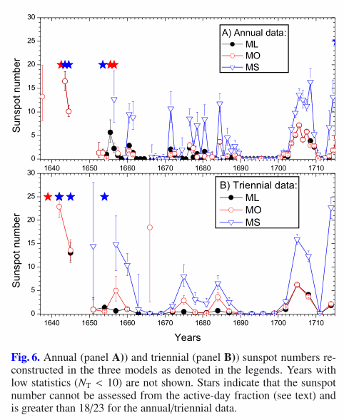
Results. A clear cyclic variability is found throughout the MM with peaks at around 1655–1657, 1675, 1684, 1705, and possibly 1666, with the active-day fraction not exceeding 0.2, 0.3, or 0.4 during the core MM, for the three models. Estimated sunspot numbers are found to be very low in accordance with a grand minimum of solar activity.
Conclusions. For the core MM (1650-1700), we have found that (1) A large portion of no-spot records, which correspond to the solar meridian observations, may be unreliable in the conventional database. (2) The active-day fraction remained low (below 0.3-0.4) throughout the MM, indicating the low level of sunspot activity. (3) The solar cycle appears clearly during the core MM. (4) The length of the solar cycle during the core MM appears for 9 ± 1 years, but this is uncertain. (5) The magnitude of the sunspot cycle during MM is assessed to be below 5–10 in sunspot numbers. A hypothesis of the high solar cycles during the MM is not confirmed.
Post by Tim

I would be interested to see Leif Svalgaard’s comments on how this paper treats the sunspot data.
Better to carefully work independently than to join a group of dull people being voluntarily misled.
Paul Vaughan says: May 9, 2015 at 5:13 am
“Better to carefully work independently than to join a group of dull people being voluntarily misled.”
Indeed! Best to listen carefully to those that admit, “I have no clue”! 🙂
Volcanic earthquakes at Mount Hakone increased their frequency on 26 April. Since then, May 4, there has been about 790 aftershocks of magnitude 2.6 on the Richter scale. But on Tuesday magnitude shocks has increased significantly, which felt Ovakudani residents in the valley.
Hakone is an extinct volcano, located 80 km from Tokyo, part of the National Park Fuji-Hakone-Izu. In its crater there are a couple of young volcanic peaks and Lake Ashi. The last time this ancient volcano erupted in 1170.
They didn’t look at C14 data. That shows a 14 year period.
David Archibald Radio flux corresponds to the change EUV. Use this page. The data from 1947.
http://www.spaceweather.ca/solarflux/sx-eng.php
“Mimo, że gęstość na wysokościach satelitarną

jest co najmniej miliard razy niższe niż na poziomie morza, na orbicie obiektów o prędkości
są tak wysokie, że nie jest jeszcze siła oporu, które można zmierzyć. Siła ta może
być obecnie pochodzą z obserwacji przestrzeni kosmicznej orbicie satelitarnej operacyjnych śledzenia
danych o wysokości do około 500 km, a za pomocą bardziej wyspecjalizowanych metod
lub sprzętu do około 1500 km. Śledzenie pomiarów na pierwszych sztucznych
satelitów [Jacchia, 1959; King-Hele 1992] doprowadziła do identyfikacji
wielu istotnych różnic w gęstości, które zostaną pokrótce tutaj “. http://esamultimedia.esa.int/docs/EarthObservation/acceldrag_finalreport_compressed.pdf
Another indicator of the level of solar activity is the flux of radio emission from the Sun at a wavelength of 10.7 cm (2.8 GHz frequency). This flux has been measured daily since 1947. It is an important indicator of solar activity because it tends to follow the changes in the solar ultraviolet that influence the Earth’s upper atmosphere and ionosphere. Many models of the upper atmosphere use the 10.7 cm flux (F10.7) as input to determine atmospheric densities and satellite drag. F10.7 has been shown to follow the sunspot number quite closely and similar prediction techniques can be used. Our predictions for F10.7 are available in a text file, as a GIF image, and as a pdf-file. Current values for F10.7 can be found at: ftp://ftp.geolab.nrcan.gc.ca/data/solar_flux/daily_flux_values/fluxtable.txt.
The lower stratosphere shows that you will not too warm in Europe (except Spain).
http://earth.nullschool.net/#2015/05/13/1200Z/wind/isobaric/70hPa/orthographic=24.35,68.24,442
ΔC14% Kocharov (1995) Vs Zolotova and/or Vaquero (2015)
Click to access aa25962-15.pdf
Observations of the Sun’s corona during the space era have led to a picture of relatively constant, but cyclically

varying solar output and structure. Longer-term, more indirect measurements, such as from 10Be, coupled by other
albeit less reliable contemporaneous reports, however, suggest periods of significant departure from this standard.
The Maunder Minimum was one such epoch where: (1) sunspots effectively disappeared for long intervals during
a 70 yr period; (2) eclipse observations suggested the distinct lack of a visible K-corona but possible appearance of
the F-corona; (3) reports of aurora were notably reduced; and (4) cosmic ray intensities at Earth were inferred to be
substantially higher. Using a global thermodynamic MHD model, we have constructed a range of possible coronal
configurations for the Maunder Minimum period and compared their predictions with these limited observational
constraints. We conclude that the most likely state of the corona during—at least—the later portion of the Maunder
Minimum was not merely that of the 2008/2009 solar minimum, as has been suggested recently, but rather a state
devoid of any large-scale structure, driven by a photospheric field composed of only ephemeral regions, and likely
substantially reduced in strength. Moreover, we suggest that the Sun evolved from a 2008/2009-like configuration
at the start of the Maunder Minimum toward an ephemeral-only configuration by the end of it, supporting a
prediction that we may be on the cusp of a new grand solar minimum.
Click to access riley_ApJ_2015.pdf
Distribution of water vapor coincides with the temperature.

lsvalgaard:

The red is sunspot areas, the blue is sunspot numbers. The reason the blue is above the red after 1846 is that the solar observers in Zurich [and Locarno] started to count big spots more than once [a really big one would be counted as five spots] which artificially inflates the sunspot number. But we can correct for that and restore the excellent correspondence between sunspot area and sunspot number.
With the UK having just had elections I am in a political frame of mind, and I must say I object to Usoskin labelling the forthcoming minimum as Eddy as seen in one of Ren’s graphs above. Eddy did not predict this minimum, the only person who’s name deserves to be on that minimum is Landscheidt.
Whilst Eddy was no doubt a significant influence on early US solar science, Landscheidt was predicting this minimum back in 1983 when no one else was and so earned his place in history.
If Leif has succeeded in getting Eddy’s name on the minimum then he has misused his stature in the solar science world to deprive Landscheidt of his due recognition.
Michele, that second graph looks like something I drew. The period between the peaks looks like the Hale Cycle and therefore the solar cycles may have been about 10 years long.
J Martin – Landscheidt’s problem was that he did not share his code. After he died, a friend of mine in Melbourne who was in contact with his widow asked me to go to the town near the Czech border where Landscheidt had lived and download the contents of his hard drive. I was preoccupied and left it too late. By the time I contacted his widow, a PhD student from Potsdam had been through and cleaned everything out. The lesson from that is that one should go get data as soon as it is offered. So if Landscheidt doesn’t have a legacy, it may be partly my fault. But he made it too difficult. You can’t reconstruct what he did from his published papers. By comparison, Ed Fix made his Excel file available as soon as his paper came out.
more convincing than Miyahara on Maunder cycle length:
Usoskin Mursula Kovaltsov (2001). Heliospheric modulation of cosmic rays and solar activity during the Maunder minimum. JGR.
Click to access 2000JA000105.pdf
Regarding Landscheidt DA wrote:
“You can’t reconstruct what he did from his published papers.”
I object sternly and with great offense to the framing.
Maybe you can’t, but I had no problem doing it all quickly (back when I was a grad student and had the luxuries of time & resources).
At first the meaning of some of Landscheidt’s terms evaded me, so I checked with a local physicist who was keenly interested but had no clue about the stats. I decided not to bother trying to understand what Landscheidt did and rather just explore. Then I noticed a 1:1 correspondence between some of the metrics I developed and Landsheidt’s “finger” & “hand” cycles. I quickly realized I had made a substantial improvement on his methods. I posted all the graphs at the talkshop, but after I left the university they deleted the contents of my account, including all of the graphs. That’s not a loss of any consequence, as it’s easy to reproduce all of that stuff from scratch.
The stuff is not complicated at all. It’s dead simple. If someone can’t reproduce it, that’s certainly informative.
–
More generally, when people beg for others’ codes, that transparently informs about independent ability (…and lack thereof). It’s an advertisement that the student cannot function without the teacher’s help, as for example would occur in an exam setting.
There’s a massive difference between being able to follow a recipe and being able to independently engineer an equivalent recipe from scratch. The former requires only a dim-wit, whereas the latter requires a formidably much higher level of intelligence.
Withholding codes is an excellent way to test competence & integrity. The ability to test students is essential to grading. You can’t test the students if forced to release the answers before the exam.
Philosophical differences on code privacy are deep and intractable. Ethically there are competing objectives, so the first sign of politics is gross oversimplification of the issue.
@David Archibald
I am perplexed why you still follow the Ed Fix model, any model that cannot hindcast the Holocene has already failed, I think you are on a loser on that one.
Your story re Landscheidt is interesting in historic terms but has no impact on the science. There is no code or secret stuff in Landscheidt history that can be divulged, his science is complete with all papers and books published.
Landscheidt used the negative extrema of solar torque to predict solar grand minima…end of story.
This method is flawed but gave us insight to the real driver.
Landscheidt method: J opposite S,U,N
The new method: J,U,N opposite S which lines up accurately with all solar slow downs.
Not forgetting the Salvador/Talkshop model, which also lines up with solar slowdowns pretty well.
Still not quite sure what the Salvador model is based on. Models can have so many inputs, I rely totally on one planetary configuration…very easy to falsify.
Hi Geoff,
Basically, it uses several planetary pair conjunction periods, modulated by other longer term planetary conjunction cycle periods and their harmonics. Details are in Rick Salvador’s PRP paper.
C14 growth indicates weakening Earth’s magnetic field.

Hi Roger,
The model is still unclear, if it is based on VEJ alignments we already know that the VEJ alignments go out of sync with SSN when J/U/N are aligned with S opposing. Tail wagging the dog?
Ian Wilson would probably agree?
ren says:
May 10, 2015 at 11:41 am
C14 growth indicates weakening Earth’s magnetic field.
ren…cough cough vuk.,
The official 14C, 10Be record is calibrated to match the changing magnetic field recorded here at Earth.
Tallbloke, re your graph above, it seems to stop in 1969. Have you got a couple of hundred years of forecast you could share with us please? If you have a forecast and your hindcast match is as good as it looks, I am prepared to worship a new god.
DA is up for a religion change it seems?
Geoff Sharp (May 10, 2015 at 10:17 am) wrote:
“Landscheidt method: J opposite S,U,N
The new method: J,U,N opposite S which lines up accurately with all solar slow downs.”
I can’t recall ever seeing this contrasted so clearly & succinctly (although it may have been equivalently stated &/or illustrated in other forms many times – or otherwise evaded my attention in the sea of communications).
That’s usually a sign that an idea has crystallized.
The effect: ~15 year shift in the timing.
My memory of Landscheidt may be a little rusty since my curiosity & focus moved elsewhere years ago, but was not his prediction 1990?
– –
I give Landsheidt due credit for this:
No matter whether wrong or right or whatever, his works strongly stirred my initial curiosity in sun-climate relations far, far more than any others. The critical utility of initial exploratory inspiration should not be underestimated. I doubt I would have taken any enduring interest in sun-climate relations were it not for early exposure to Landscheidt’s works.
It’s vacuous in the aesthetic eastern sense of the way: Landscheidt simply built a mystery that critically hooked imaginations, thus securing the powerfully educational “Landsheidt Minimum” legacy.
I’ve previously suggested replacing “Grand” with “Eddy”, such that collectively all Grand Minima become known as “Eddy Minima”. (There’s nothing grand or indispensable about “Grand”.)
Hi David: Here’s the model’s hindcast and forecast to 2100 for sunspot numbers. Clearly the current cycle 24 and following cycle 25 are overestimated since our model is not yet sufficiently sophisticated to deal with the non-linearities. Tim Chanon and I have been discussing how we might work an additional ‘subroutine’ in to handle that.
Note that if correct, this means we get 1970’s levels of activity for half a century after the ‘recovery’ from the expected grand minimum. However, also note how the model fails to capture the full amplitude of some higher cycles following the Dalton minimum.
By the way, the dTSI 10Be data actually extends to the 2000AD, past 1969. The X-Axis labelling leaves a little to be desired.
Paul, yes Landscheidt was 20 years out and much further with other grand minima events. He had the wrong configuration, but was close.
tallbloke says:
May 10, 2015 at 12:34 pm
The model is not looking good really, SC20 is totally missed which is a major flaw.
Geoff, there’s nothing unclear about the Salvador model. It has been discussed in extensive detail at the talkshop (during collaborative development). The later paper spells everything out in exacting detail …but the naturally meandering talkshop discussion record is easier (and far less stale) to follow. There’s even an excel spreadsheet with all the calculations. I’ve reproduced all of the results using wavelets and determined that the model can be improved with due attention to SCL & SCD (solar cycle length & deceleration …or solar cycle frequency & frequency-shift, if you prefer). It’s a trivial exercise to extend the 10Be framework to model the d18O Dansgaard-Oeschger center manifold. (To my knowledge Salvador has not done this yet and may not yet be aware.)
Paul, lets discuss it now in full detail. Give us the formula (model) that is behind the Salvadore curve.
Lol! Geoff, that’s not my role. You can independently look up (a) the 2 talkshop threads where the model was developed and (b) Salvador’s paper. You can also simply get the excel spreadsheet!!
I’ll add 1 clarification: The model passes lots of tests, but it fails diagnostics on SCL & SCD (…so that’s a clear clue about where it needs improvement).
It will be interesting to see if RJ follows the tips I’ve left in suggestions-10 (with spillover into suggestions-11) about how to extend the model to d18O 1470.
Modeling doesn’t interest me at all. I’ll just keep reporting insights from explorations. What modelers do with such observations is their call.
Paul Vaughan says: May 10, 2015 at 12:51 am
“Withholding codes is an excellent way to test competence & integrity. The ability to test students is essential to grading. You can’t test the students if forced to release the answers before the exam.”
For computational models it is the code itself not the results that decide the worth! My morning and early afternoon work was well commented for understanding by others. By 8PM trying to get the damn thing to work, no comments, no understanding even by me. Raw mistakes that resulted in raw error, but are still in use today, by climatologists!
“Philosophical differences on code privacy are deep and intractable. Ethically there are competing objectives, so the first sign of politics is gross oversimplification of the issue.”
Indeed that is so the yet unborn can vote for your continuance! No politician wishes any to understand!
It is always, Trust me, at this State Fair I offer the only set of knives that never get dull 🙂
No probs Paul, if you are not up to the task. I am just asking for a clear explanation of the Salvadore model, instead of leading us all astray perhaps you could clearly explain how it exactly works?
Other wise is it clearly Willis fodder?
Geoff, I’m not here to promote the Salvador model, nor am I hear to lead anyone astray.
If people can’t independently recognize which insights can be taken to the bank versus what material is simply designed to promote further exploration, that’s informative.
The 4 hyperlinks you seek are 1 quick web search away if you can’t tell the difference yet.
As for wuwt, the only commentator there worth reading is Bill Illis. I do recall seeing him err quite seriously once, but aside from that he has given a lot of useful tips.
If you want to discuss something really solid, there’s something of that nature in suggestions-11 in response to Ian Wilson’s comment on multi-fractals.
Geoff Sharp
The earth’s climate has been significantly affected by the planet’s magnetic field, according to a Danish study published Monday that could challenge the notion that human emissions are responsible for global warming.
“Our results show a strong correlation between the strength of the earth’s magnetic field and the amount of precipitation in the tropics,” one of the two Danish geophysicists behind the study, Mads Faurschou Knudsen of the geology department at Aarhus University in western Denmark, told the Videnskab journal.
He and his colleague Peter Riisager, of the Geological Survey of Denmark and Greenland (GEUS), compared a reconstruction of the prehistoric magnetic field 5,000 years ago based on data drawn from stalagmites and stalactites found in China and Oman.
The results of the study, which has also been published in US scientific journal Geology, lend support to a controversial theory published a decade ago by Danish astrophysicist Henrik Svensmark, who claimed the climate was highly influenced by galactic cosmic ray (GCR) particles penetrating the earth’s atmosphere.
Svensmark’s theory, which pitted him against today’s mainstream theorists who claim carbon dioxide (CO2) is responsible for global warming, involved a link between the earth’s magnetic field and climate, since that field helps regulate the number of GCR particles that reach the earth’s atmosphere.
“The only way we can explain the (geomagnetic-climate) connection is through the exact same physical mechanisms that were present in Henrik Svensmark’s theory,” Knudsen said.
“If changes in the magnetic field, which occur independently of the earth’s climate, can be linked to changes in precipitation, then it can only be explained through the magnetic field’s blocking of the cosmetic rays,” he said.
http://phys.org/news/2009-01-earth-magnetic-field-impacts-climate.html
Will, I’m not talking about crazy models. They aren’t worthwhile. I’m talking about simple, straightforward algorithms.
Not good enough Paul, simple question, but no answer.
But there is probably no point, as the model predicts the Dalton Minimum but misses SC20 and SC24 and beyond. Nothing else needs to be stated.
My model is simple…J/U/N with S opposed, when it happens the Sun slows down…prove me wrong?
ren/vuk,
Your reply is not relevant. Earth’s changing magnetic field is calibrated (allowed for) in the 14C and 10Be solar proxy record.
ren has pointed to this 2009 paper:
Is there a link between earth’s magnetic field and low-latitude precipitation?
Click to access 71.pdf
Once again it looks like insolation pattern affects the magnetic field by redistributing water pressure.
May 9, 2015 at 11:31 pm
William M. Gray
Professor Emeritus
Colorado State University
The model simulations have followed the unrealistic physical ideas emanating from the National Academy of Science (NAS), 1979 (or Charney Report). This report speculated that as the troposphere warms from CO2 increases that this warming would be accompanied (follow the Clausius-Clapeyron relationship between temperature and moisture) by a moisture increase such that the relative humidity (RH) of the air would remain near constant as the temperature increased. Implicit in this NAS assumption of CO2 induced warming was the necessity that this increase of moisture would add additional blockage of infrared (IR) radiation to space beyond what the CO2 gas did by itself. The net IR blockage to space from increasing CO2 was thus assumed to occur not only from the CO2 gas itself but also from the extra water-vapor gain needed to keep the RH near constant as the temperature rose. This additional water-vapor gain was shown by the models to have about twice as large an influence on reducing IR blockage to space as the CO2 increase by itself. Thus, any CO2 increase of one unit of IR blockage to space would simultaneously bring along with it an additional two units of water-vapor blockage of IR loss to space. This additional moisture related blockage of IR loss to space (associated with CO2 induced warming) has been designated as ‘positive water-vapor feedback’. All the CO2 climate models have strong amounts of positive water-favor feedback.
It is this large and direct tie of water-vapor increase with CO2 induced temperature rise which is the primary physical flaw in all of the GCM CO2 doubling model simulations. This is the reason why all the GCMs have so strongly over-predicted the amount of global warming which will occur with a doubling of atmospheric CO2.
Observations show that the warming or cooling of the upper troposphere does not occur with RH remaining close to constant. Temperature and RH tend to change oppositely from each other and not in unison as the models assume. My project’s study of cumulus convection and tropical cyclone formation over many decades has taught me that the NAS 1979 (Charney) Report assessment that rising CO2 amounts will occur with water-vapor increase is not a realistic assessment of how these parameters change in the upper troposphere.
The GCM CO2 simulations are also constructed so as to have their moisture simulations arranged such that water-vapor changes occur uniformly at both upper and lower tropospheric levels. By contrast, the observations of moisture change at upper and lower tropospheric levels show them to be little related to each other (Figure 3).


Our project’s many years of analysis of the International Satellite Cloud Climatology Project (ISCCP) observations of IR loss to space in association with enhanced Cb convection and rainfall do not show a decreased IR blockage to space (as the models have indicated will occur) but rather an enhancement of IR loss to space. Our data analysis is, by contrast with the models, representation of a negative water-vapor feedback – the larger the rainfall rate, the lower the upper tropospheric water-vapor content and the greater the IR loss to space (Figure 6).
https://stevengoddard.wordpress.com/2015/05/09/dr-bill-gray-explains-why-climate-models-dont-work/
The Earth’s magnetic field has been sliding over the entire Holocene. If you look at the raw isotope data it follows the same downward trend overall. But once the changes in the Earth’s magnetic field are adjusted out, the true picture of solar activity emerges.
That picture once adjusted shows the power of the Sun compared with solar grand minima across the Holocene, which is directly related to the position of Saturn when Jupiter, Uranus and Neptune are opposed. This position controls the timing and power of all solar grand minima.
Once again…if anyone can prove me wrong?
With graphics follows that around 1970 there was a sharp increase in C14 and further was very high, despite strong cycles 21,.22. Am I wrong?

19 June 2014
The first set of high-resolution results from ESA’s three-satellite Swarm constellation reveals the most recent changes in the magnetic field that protects our planet.
Launched in November 2013, Swarm is providing unprecedented insights into the complex workings of Earth’s magnetic field, which safeguards us from the bombarding cosmic radiation and charged particles.
June 2014 magnetic field
Measurements made over the past six months confirm the general trend of the field’s weakening, with the most dramatic declines over the Western Hemisphere.
But in other areas, such as the southern Indian Ocean, the magnetic field has strengthened since January.
The latest measurements also confirm the movement of magnetic North towards Siberia.
These changes are based on the magnetic signals stemming from Earth’s core. Over the coming months, scientists will analyse the data to unravel the magnetic contributions from other sources, namely the mantle, crust, oceans, ionosphere and magnetosphere.

http://www.esa.int/Our_Activities/Observing_the_Earth/Swarm/Swarm_reveals_Earth_s_changing_magnetism
Paul Vaughan says: May 10, 2015 at 2:30 pm
Will, I’m not talking about crazy models. They aren’t worthwhile. I’m talking about simple, straightforward algorithms.
OK! Straightforward algorithms of what? What kind of geometry?
I was commenting on the so called “LBLRTM” Line-By-Line Radiative Transfer Model. The most insidious fuckup of all science. The HiTran database is a field verified attenuation, by species, of spectral temporal/spatial modulation of EMR. It was done at obscene cost, to characterise the impediment to atmospheric “seeing” at various wavebands and distances. (If we can’t see them, they cant see us either), unless they are schmart! It has nothing at all to do with any atmospheric storage of the illogical radiant heat from the surface.! The idiots wish to claim such “causes” “warming”, whatever that may mean! 🙂
Geoff,
Links for your JVN -S graph, also a link for your ‘earths magnetic field adjusted out’ graph. Please and thank you.
Its a shame no one carried on Landscheidts work. Many people seem to think he was on to something. 1983. 1990. I didnt check, was just going on memory, but will check later.
Geoff S: My model is simple…J/U/N with S opposed, when it happens the Sun slows down…
That’s not a model, it’s an observation concerning a correlation. The Salvador/Talkshop model not only captures solar slowdowns well, it also captures upswings, meanders, wobbles and their *magnitudes* well.
“Willis fodder”
Lol. The extent of Willis’ understanding of orbital resonance and harmonics would fit in the mind of a goldfish. To borrow a phrase from HHGTTG, I don’t give a feotid pair of dingo’s kidney’s what Willis thinks. And nor should anyone else where astrophysics, solar system dynamics and solar-terrestrial relations are concerned.
Over here, WIllis and Mosher’s petulant demands to be spoonfed data and code in the bitesize dollops of their preference get laughed at. After WUWT’s siding with the censors at Copernicus and their libellous assault on the eminent scientists we published alongside, they can whistle.
.
tallbloke says: May 10, 2015 at 4:12 pm
(“Geoff S: My model is simple…J/U/N with S opposed, when it happens the Sun slows down…”)
“That’s not a model, it’s an observation concerning a correlation. The Salvador/Talkshop model not only captures solar slowdowns well, it also captures upswings, meanders, wobbles and their *magnitudes* well.”
Any computer model only repeatedly and precisely produce a repeat of ignorance. Computers are very good at that. Please defend your Salvador/Talkshop model as different? 🙂
Tallbloke, thankyou very much. To my eye, it looks like a Dalton Minimum repeat and then 19th century-like from there. Now back to the graph that goes back to -2000 AD, do you have that going out to say 2300 AD? I would like to see if there are any Dark Ages-type spikes down coming along. If we have hundreds of years of Minoan Warm Period-like conditions coming, that is not very scary. Once again, thanks for enlightening me.
From the Salvadore paper:
This model is simply four interacting waves, but they are
modulated to create an infinite possibility for sunspot for-
mation.
The basic frequencies in years are:
–
a VEJ frequency of 22.14 (varying),
–
a VEJ frequency of 19.528 (varying and forming a beat
frequency of 165.5 with 22.14),
–
Jupiter–Saturn synodic frequency of 19.858,
–
one-quarter Uranus orbital frequency equal to 21.005,
–
two modulating frequencies of 178.8 and 1253 (forming
a beat frequency of 208 yr).
————————————————————–
With that many inputs you are bound to get some of it right over short time frames. But there is one glaring problem with the Salvadore model, there is no 208 year cycle but instead there is a most common gap of 208 years between grand minima over the Holocene. During the LIA the gap was much less, so this model will fail over the longer term. McCraken et al 2014 understand this completely.
My correlations is of course not a model, I do not need a model, one need only observe the AM or solar distance graph and look for the “barycentric anomalies” (McCraken et al 2014). A model could be built but it would have to include much data and several parameters, maybe someone will have a go at it someday.
tallbloke says:
May 10, 2015 at 4:12 pm
That’s not a model, it’s an observation concerning a correlation. The Salvador/Talkshop model not only captures solar slowdowns well, it also captures upswings, meanders, wobbles and their *magnitudes* well.
The model misses SC20 and SC24, so does not capture solar slowdowns. This is a fatal error?
J Martin says:
May 10, 2015 at 4:09 pm
Geoff,
Links for your JVN -S graph, also a link for your ‘earths magnetic field adjusted out’ graph. Please and thank you.
Its a shame no one carried on Landscheidts work. Many people seem to think he was on to something. 1983. 1990. I didnt check, was just going on memory, but will check later.
The J/U/N -S graph is simply Carls graph…look for the green arrows.
Any 14C graph (INTCAL98 onward, Solanki, Usoskin etc) incorporates the Earth’s magnetic field calibrated out. I have seen the raw 14C record but will need to search for it.
Landscheidts work has been continued by, Carl Smith, myself and McCracken, Beer and Steinhilber. Landscheidt had it wrong (red dots on Carl’s graph) but he gave us the gateway to discover the ultimate key to solar grand minimum (green arrows).
ren says:
May 10, 2015 at 3:39 pm
With graphics follows that around 1970 there was a sharp increase in C14 and further was very high, despite strong cycles 21,.22. Am I wrong?
Because of the atomic bomb all 14C data is rendered useless after 1945.
Note to the PHP editors: There is a mistake in the Salvadore paper. In the text and references the “thetemperstspark” data is wrongly associated with myself.
David A: do you have that going out to say 2300 AD?
Hi David. We won’t release a longer projection of the model until we’ve addressed the issues I pointed out with non-linearities around cycle 24/25.
Geoff S: Landscheidt had it wrong
In fact, Landscheidt also predicted a solar grand minimum centred on 2035.
The model misses SC20 and SC24, so does not capture solar slowdowns. This is a fatal error?
The model captures the major solar slowdowns of the LIA (and others back to 2000BC) extremely accurately, so no, it’s not a fatal error. I’ll certainly consider working the working the JUN-S dynamic into the model to see if it helps improve the 1970 & SC24/25 situation.
Salvadore
The man’s name is Salvador.
Note to the PHP editors: There is a mistake in the Salvadore paper. In the text and references the “thetemperstspark” data is wrongly associated with myself.
I already apologised to Sparks for the error. Shit happens.
Landscheidt and others who used his method also predicted a solar grand minimum for 1990, the later prediction for 2030 is probably a bit late. The facts are that he used the wrong planetary configuration.
Rog, you have used two models in this thread, none predict SC20 & SC24..Can you provide the data (inputs) for the Salvador TSI model? I was commenting on the other model (ie the one that is similar to the Salvador paper).
Apologies to Salvador.
Geoff Sharp says:
“Rog, you have used two models in this thread, none predict SC20 & SC24”
But perhaps it is no coincidence that in Cycle 20 so increased the level of C14?
The chart shows that approximately 40%.
Abstract
The Maunder Minimum was the time during the second part of the 17th century, nominally from 1645 to 1717 AD, when unusually low numbers of sunspots were observed. On the basis of numerous recorded observations of auroras in the early 18th century, the end of the Minimum could be regarded as around 1700, but details of sunspot observations by Jan Heweliusz (Heweliusz, Machina Coelestis, 1679), John Flamsteed and Philippe de La Hire in 1684 allow us to interpret the Maunder Minimum as the period without a significant cessation of activity. This Minimum was also recognized in 14C data from trees which grew during the second part of 17th century. The variation in the production rate of radioactive carbon isotope 14C is due to modulation of the cosmic ray flux producing it by the changing level of solar activity and solar magnetic flux. Stronger magnetic fields in the solar wind make it more difficult for cosmic rays to reach the Earth, causing a drop in the production rate of 14C. However, more detailed analyses of 14C data indicate that the highest isotope abundances do not occur at the time of sunspot minima, as would be expected on the basis of modulation of the cosmic ray flux by the solar magnetic field, but two years after the sunspot number maximum. This time difference (or phase delay) can be accounted for if in fact there are both solar and non-solar cosmic ray contributions. Solar flares could also contribute high-energy particles and produce 14C and are generally not most frequent at the time of the highest sunspot numbers in the cycle. Solar flares, most frequent about two years after the sunspot maximum, could be the main source of increased 14C isotope abundance. This idea changes established earlier relations between sunspot number of this time regarded as low and increased abundance of 14C isotope, and allows us to interpret the Maunder Minimum as a botanical or statistical effect.
http://adsabs.harvard.edu/abs/2010SoPh..261..337R
If the Earth’s magnetic field is weakening or it could affect the production of solar protons C14?
Geoff, quantifying S opposite JUN is easily feasible. It’s concerning that you don’t seem to be aware of the longer JEV cycle with period N. Perhaps the prolonged conflicts you’ve endured with hostile enemies have shortened your temper, impacting your faith in the possibility of cordial exchange & good will. Please be reassured that when time & resources permit, I will look into the confounding of your observations with N-period JEV supercycles. The confounding provides a bridge between frameworks. Salvador’s model is flexible as is Salvador’s mind. He’s nothing like the bitter enemies you’ve fought in hostile, ignorant, thought-policed arenas.
Thanks Paul, I am aware of the JEV alignments and solar cycle length but am not really too impressed by a mixture of cycles placed in a model that once tweaked does some curve matching of the past. While possible I also think the physical forces and amount of change are just too weak for JEV to have an impact on grand minima without some help from the big four.
But having said that the dTSI model of Salvador does look very impressive on the face of it, but wonder exactly how the result is reached. Rog and yourself are saying the detail is in his paper but the dTSI graph and the other graphs in his paper bear no resemblance…surely they are not all coming from the same piece of code?
I am particularly interested in how the match to past grand minima is achieved especially since gaps between grand minima can be 90-210 years approx and much greater when we miss altogether as in the MWP. A model based on my theory and McCracken et al could do that as it knows the gaps exactly as it can test the alignment strength of JUN-S which not only would get the timing right but also the depth of each part of the slowdown (for the most part as cycle timing also comes in to play). That would take some pretty fancy code using my theory, so I am wondering how Salvador has managed it?
Geoff,
Here are a few comments to provide some context to the models.
These models are works in progress and for me a model is not reality. Reality is much more complicated than any model. But a simplified model may help us better understand reality if it has reasonable predictive properties. When the model presented in my paper was constructed your paper on JUN-S and Ian Wilson’s on SOC, spin orbital coupling, had not been published and the thinking behind them was unknown to me. I saw your paper as I was writing mine and I referenced it as you pointed out the significance of the Jupiter synodics with the other large gas giants.
The first model covered 1000 years and was constructed with the help of time frames indentified by Solanki C14 sunspot data for solar minimums. The model is simple by design so we can understand it, but with four frequencies it is limited to 1000 years.
I thought I could extend the time frame of the model based on the SOC of Ian Wilson and your work based on the conjunction of Jupiter synodics. This added two more frequencies the SOC of 22.38 and the JN synodic of 2 times 12.782. I left the one quarter Uranus for reasons of solar system resonance instead of the J/U synodic. This second model, a 6 frequency model, required better data than Solanki so I used Steinhilber/ Mckracken dTSI for solar activity. This model does a fair job for 4000 years and gives predictions for solar minimums. (2027 to 2045) & (2132-2147). Is it right? Time will tell.
I think that your work which identifies the key importance of the conjunction of gas giants along with Ian Wilson’s VEJ-SOC and Nicola Scafetta’ resonance is probably the basis for a relatively simple model which will describe the entire Holocene.
Other life issues have intervened so I’m not getting much time to look at this further but I thought I should clarify.
Bests of luck to you.
Rick
Thanks very much Rick, I think without your intervention I would still be in the dark. It was pretty clear to me that the two models could not be a product of the same source. Personally I think your 2nd attempt is more robust than the 1st.
My theory has been around since 2008 on the web, it was first published in 2010 (arxiv) and then finally peer reviewed in 2013. McCracken et al in Solar Physics 2014 was later published after 18 months in review with the same basic theory. Not many people are aware or understand the JUN-S theory and to date it has not been properly discussed on the Talkshop IMHO. (the McCracken version is still behind a paywall).
I am very interested in your dTSI version although I still can’t see how you made it work so well. But if it somehow has picked up the important core trends it can be independently used to test the Holocene proxy records which I think has one major flaw.
If you subscribe to solar planetary forcing there is a simple test. It doesn’t matter what planetary theory floats your boat, but what ever the theory it must reproduce itself every 4627 years. Some allowances need to be made as the proxy data is not to a fine resolution and I think the planetary force is independent of the solar cycle so timing can be an issue, but on the whole, large scale events during the Holocene should repeat every 4627 years. The Babcock crew will be onto this in the future no doubt. I have the 20,000 year solar distance to SSB (Steinhilber) ephemeris kindly forwarded on by Ken McCracken that tests the 4627 cycle, there is no doubt about the accuracy of the 4627 cycle which is probably the only true cycle when discussing the outer 4. Any theory that can’t pass the 4627 rule will fail IMHO.
If you ran your dTSI model back further we could test it against a 340 year dating error in the proxy records that I suspect is around 2800BC along with a large isotope excursion in the record that does not look to be solar induced. Your model should find the same results?
Back in 2009 I did a model run of sorts to predict (on a rough scale) future solar grand minima to 3000AD. I simply came up with a JUN-S calibration scale and then summed each occurrence of JUN-S per U/N conjunction. This gave a weighted score that is plotted at each grand minimum centre (GM). I would be interested to see your dTSI model out to 3000AD to compare.
Please feel free to contact me anytime (landscheidt.info), I would be more than happy to correspond.
Geoff
I should have stated that the 4627 year test only applies to planetary theories relying on the outer 4 planets.
[…] Fonte : https://tallbloke.wordpress.com/2015/05/08/level-and-length-of-cyclic-solar-activity-during-the-maun… […]
Geoff,
A few points of clarification:
1. The 90 year, 205 year, 165 year, & 1470 year JEV supercycles are NOT independent of jovian influence, so there has been some (quite serious) misunderstanding. I’m concerned that the community remains insufficiently aware of these cycles.
2. The succinct statement you made above clarified the root of many misunderstandings that have occurred over the years. Charvatova’s 1980s summaries are mathematically equivalent by reflection symmetry. Same applies to 1990s Fairbridge. Whenever I find time, it will only take a single sitting to do the trivial calculations.
We just have to laugh at the ridiculous number of misunderstandings that arise in discussions.
This graphic follows the path of the Sun versus the solar system barycentre (SSBC) for two periods, the first one being around the time of the Maunder minimum, the second starting in 1980. The red circle is one solar diameter away from the SSBC [click to enlarge]. Note the similarity.
Paul, you are also giving me insights. After 7 years you are still not aware of this:
If someone like you is missing the important detail I can see I have a lot in front of me. In July I am doing my first large presentation, perhaps this will be a better method of getting the word out.
I know you are a big fan of Charvàtovà and rightly so, her work is the closest to being correct IMO. But she made several mistakes and bad predictions because she did not go to the next level, so she was generally ignored. In a nutshell she knew grand minima happened within a 120 year window but never had a handle on what caused the disordered orbit pattern over that timescale.
Basically grand minima can only occur during or near the U/N conjunction, it cannot occur on the U/N opposition. McCracken et al show this in their paper using the top 20 grand minima of the Holocene (it applies to all grand minima). This in itself is supreme data that is hard to argue against, the planets have to be the driver of grand minima.
Notice the blue areas, these are the JUN-S alignments that are strong enough to cause grand minima. They only occur in the Charvàtovà disordered orbit window. The variability should make it clear that precise cycles are not in play, with 90-130-170-210 year being possible cycle repeats. The angle of Saturn is what controls the strength of the small disordered orbit that happens on average 3 times in the Charvàtovà 120 year phase and I would think this process almost impossible to detect via simple mathematics. Hence my aversion to all the cycle talk.
So in effect I and McCracken et al have verified Charvàtovà’s basic theory, but we have identified and quantified the small 10 year orbits that throw out her balanced trefoil pattern making it far more precise. The JUN-S alignment does it all.
I have emailed her several times but as yet no reply.
It is pretty obvious the PRP reviewers (Rog being one) of the latest Charvàtovà paper did not understand the JUN-S function or it would have been passed on to her?
The detail is all in the paper: http://www.scirp.org/journal/PaperInformation.aspx?paperID=36513&#reference
Oldbrew: you are catching on. The inner loop orbits causing the slowdown are both from the JUN-S alignment happening in your diagrams. The first version of Arnholm’s software shows it a lot clearer.
The orbit during the Maunder (1650) is stronger than 2010 and is also followed up 40 years later with another fairly strong orbit. There is NO second disordered orbit this time (2050) around showing the big difference between the two epochs and why we wont have another Maunder Minimum for at least a 1000 years. The Saturn angle once again being the key.
Btw the 1470 year cycle is JSN i.e. 74 J-S, 115 J-N, 41 S-N.
Also 8.92 N, 49.92 S, 123.92 J – note the same decimal value.
Geoff Sharp (May 13, 2015 at 12:06 am) suggested:
“you are still not aware of this”
It has been on the backburner along with a long list of other things. I operate on the Pareto Principle. I wait for the revelation that makes solution easy. The super-concise comparison you made with Landscheidt’s framework (one I know inside-out) gave me instant translation, making now the time to efficiently rotate the priority level back up.
–
Geoff Sharp (May 13, 2015 at 12:06 am) suggested:
“I would think this process almost impossible to detect via simple mathematics”
I’ve worked out the geometry. Simple quantification is easily feasible. (Long ago I knew that would be the case if ever / whenever the exercise secured priority.)
–
Update:
I’ve developed both amplitude & phase measures of the degree to which S is opposite JUN.
–
…and as should be obvious to anyone who understands that we’re in the realm of trivial geometric proofs:
There’s perfect correspondence with the green & red arrows Geoff put on Carl’s AM graphs.
Geoff Sharp (May 13, 2015 at 12:06 am) suggested:
“you are still not aware of this”
It has been on the backburner along with a long list of other things. I operate on the Pareto Principle. I wait for the revelation that makes solution easy. The super-concise comparison you made with Landscheidt’s framework (one I know inside-out) gave me instant translation, making now the time to efficiently rotate the priority level back up.
–
Geoff Sharp (May 13, 2015 at 12:06 am) suggested:
“I would think this process almost impossible to detect via simple mathematics”
I’ve worked out the geometry. Simple quantification is easily feasible. (Long ago I knew that would be the case if ever / whenever the exercise secured priority.)
–
Update:
I’ve developed both amplitude & phase measures of the degree to which S is opposite JUN.
–
…and as should be obvious to anyone who understands that we’re in the realm of trivial geometric proofs:
There’s perfect correspondence with the green & red arrows Geoff put on Carl’s AM graphs.
I’ve deleted all the work I just did.
I’ll redo the work and share it if/when community members understand and acknowledge the multidecadal regional aberration proofs I’ve shown based on SCD and decadal cyclic volatility of semi-annual earth rotation. 1+1=2 needs to be understood and acknowledged.
Regards
In the long term a J-U-N triple conjunction should repeat every 22 U-N. As that’s ~3771 years it can’t be demonstrated on the solar simulator (3000 year limit) but the half period shows J opposite U-N so it looks OK.
Paul, there is more to understand. The angle of Saturn is the key to the amount of solar disruption with a most disruptive angle of +30 to +40 deg being the strongest, Saturn directly opposite being weak (SC20) and then getting weaker as we get on the negative side (see diagram). You also have to allow for the distance between U/N with together the strongest and around 60 deg apart for a result. The Saturn angle controls where the perturbation of the the AM occurs and also the shape of the 10 year disordered orbit.
There is more but that will cover around 90% of grand minima across the Holocene.
Geoff Sharp (May 13, 2015 at 11:57 pm) suggested:
“Paul, there is more to understand.”
Geoff, there’s more to understand. Better head on over to Suggestions-11.
Geoff Sharp (May 13, 2015 at 11:57 pm) suggested:
“There is more but that will cover around 90%”
Indeed, 90% of multidecadal-centennial climate variation is sun-driven.
also:
10% = ENSO
~0% = CO2
– — –
Geoff Sharp (May 13, 2015 at 11:57 pm) suggested:
“The angle of Saturn is the key to the amount of solar disruption with a most disruptive angle of +30 to +40 deg being the strongest, Saturn directly opposite being weak (SC20) and then getting weaker as we get on the negative side (see diagram). You also have to allow for the distance between U/N with together the strongest and around 60 deg apart for a result. The Saturn angle controls where the perturbation of the the AM occurs and also the shape of the 10 year disordered orbit.”
As indicated, I’ve already done this. It’s a breeze to pinpoint the optimal angle.
Paul Vaughan says:
May 14, 2015 at 8:30 am
As indicated, I’ve already done this. It’s a breeze to pinpoint the optimal angle.
If you have already created a model that can do this I am very impressed. If you compare the model run to the Steinhilber 10Be you should get a very good result. If correct there should be anomalies at
573BC, 2850BC and after 2500BC the records need to be adjusted by 340 years.
It’s not a “model run”. It’s a few columns of trivial calculations.
Now: I need a new puzzle to work on….
How about: ‘Atmospheric electricity, considered in a general manner, attains its maximum in January, then decreases progressively until the month of June, which presents a minimum of intensity; it increases during the following months to the end of the year.’ –
http://en.wikipedia.org/wiki/Atmospheric_electricity#Variations
Which matches perihelion (Jan.) and aphelion (July). So maybe no puzzle 😉
Anyone doing the calculations independently can start with output from:
http://ssd.jpl.nasa.gov/horizons.cgi
I’m linking to figure 8 from Geoff’s paper to make it easier to find for discussion at a future date:

Good timing as that diagram shows new information discovered post the paper. The AMP angular momentum perturbation types have been reclassified. There is now type “A” “B” and “C”, A is when Saturn is between 0 and +40deg (approx) which affects the first part of the disordered inner loop (strong) and “B” is when Saturn is between -40 and 0 and affects the latter half of the disordered inner loop (weak).
The new type “C” (1540AD) is not very common and is also a different planetary alignment, it requires J/S together and U/N together directly opposed and affects the outer loop path so that the Sun orbits the SSB like on a string.
This orbit creates constant AM with associated constant speed and seems to correlate with decent solar slowdowns, so there is a very good chance that this alignment is also a player.
If one was going to produce a model this configuration would also be useful. Whoever does produce this model will one day make a name for themselves, I believe.
J-3S+U+N
2545.348317 years
I don’t think anyone deserves fame for proving where straight lines intersect.