


throughout the Holocene based on Jupiter–Saturn tidal frequencies plus the
11-year solar dynamo cycle
Journal of Atmospheric and Solar-Terrestrial Physics
- Nicola Scafetta
- ACRIM (Active Cavity Radiometer Solar Irradiance Monitor Lab) & Duke University, Durham, NC 27708, USA
- Received 29 October 2011. Revised 17 February 2012. Accepted 22 February 2012. Available online 8 March 2012.
Abstract
The Schwabe frequency band of the Zurich sunspot record from 1749 to 2011 is found to be made of three major cycles with periods of about 9.98, 10.9 and 11.86 years. The side frequencies appear to be closely related to the spring tidal period of Jupiter and Saturn (range between 9.5-10.5 years, and median 9.93 years) and to the tidal sidereal period of Jupiter (about 11.86 years). The central cycle may be associated to a quasi 11-year solar dynamo cycle that appears to be approximately synchronized to the average of the two planetary frequencies. A simplified harmonic constituent model based on the above two planetary tidal frequencies and on the exact dates of Jupiter and Saturn planetary tidal phases, plus a theoretically deduced 10.87-year central cycle reveals complex quasi-periodic interference/beat patterns. The major beat periods occur at about 115, 61 and 130 years, plus a quasi-millennial large beat cycle around 983 years. We show that equivalent synchronized cycles are found in cosmogenic records used to reconstruct solar activity and in proxy climate records during the entire Holocene (last 12,000 years) up to now. The quasi-secular beat oscillations hindcast reasonably well the known prolonged periods of low solar activity during the last millennium such as the Oort, Wolf, Spörer, Maunder and Dalton minima as well as the seventeen ∼115-year long oscillations found in a detailed temperature reconstruction of the Northern Hemisphere covering the last 2000 years. Finally, the harmonic model herein proposed reconstructs the prolonged solar minima that occurred during 1900–1920 and 1960–1980 and the secular solar maxima around 1940–1950 and 1995–2005, which agrees with some solar proxy model and with the ACRIM TSI satellite composite. The model forecasts a new prolonged solar minimum during 2020–2040, which is stressed by the minima of both the 61 and 115-year reconstructed cycles. Finally, the model predicts that during low solar activity periods, the solar cycle length tends to be longer, as observed in solar and climate proxy records. These results clearly indicate that both solar and climate oscillations are linked to planetary motion and, furthermore, their timing can be reasonably hindcast and forecast. The demonstrated geometrical synchronicity between solar and climate data patterns with the proposed solar/planetary harmonic model rebuts a major critique (by Smythe and Eddy, 1977) of the theory of planetary tidal influence on the Sun. Other qualitative discussions are added about the plausibility of a planetary influence on solar activity.
► Holocene-to-now solar dynamics is hindcast with Jupiter/Saturn/Schawabe harmonics. ► Holocene-to-now climate variability is reconstructed with the same harmonics. ► Major natural beat harmonics with period 61, 115, 130 and 983 years are discovered. ► Oort, Wolf, Sporer, Maunder and Dalton solar grand minima (ice-ages) are explained. ► A new grand solar minimum (climate cooling?) is expected to occur in 2020-2045 A.D.
Keywords
- Planetary theory of solar variation;
- Coupling between planetary tidal forcing and solar dynamo cycle;
- Reconstruction and forecast of solar and climate dynamics during the Holocene;
- Harmonic model for solar and climate variation at decadal-to-millennial scale.
A few of the figures:

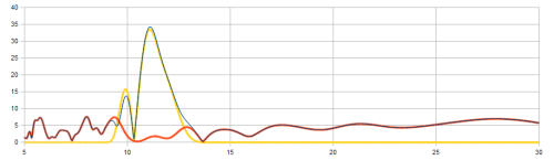
Figure 6 [C] Solar cycle length predicted by the harmonic model against the observed one (see Table 1).
Note that the model usually predicts longer solar cycles during periods of lower solar activity as it has been observed during the Maunder and Dalton minima.
[D] The solar/planetary model against the global surface temperature (HadCRUT3, http://www.cru.uea.ac.uk/) and the annual average ACRIM total solar irradiance (TSI) satellite composite (http://acrim.com/) since 1981 (note that ACRIM1 started in February/1980). Note the schematic similitude of the modulation of the patterns with local maxima around 1880, 1940 and 2000, local minima around 1910 and 1970, and the similar upward trending since the Dalton solar grand minimum.The preliminary temperature forecast (yellow) area is made with the model proposed in Scafetta (in press) plus a 115-year cycle with amplitude 0.1 o C.

Fig. 7. Modulated three-frequency harmonic model, Eq. (8), (which represents an ideal solar activity variation) versus the Northern Hemisphere proxy temperature reconstruction by Ljungqvist (2010). Note the good timing matching between the millenarian cycle and the seventeen 115-year cycles between the two records. The Roman Warm Period (RWP), Dark Age Cold Period (DACP), Medieval Warm Period (MWP), Little Ice Age (LIA) and Current Warm Period (CWP) are indicated in the figure. At the bottom: the model harmonic (blue) with period P12=114.783 and phase T12=1980.528 calculated by means of regression; the 165-year smooth residual of the temperature signal. The correlation coefficient is r0=0.3 for 200 points, which indicates that the 115-year cycles in the two curves are well correlated (P(|r|≥r0)<0.1%). The 115-year cycle reached a maximum in 1980.5 and will reach a new minimum in 2037.9 A.D.

Fig. 8. Comparison between carbon-14 (14C) and beryllium-10 (10Be) nucleotide records, which are used as proxies for the solar activity, and a composite (HSG MC52-VM29-191) of a set of drift ice-index records, which is used as a proxy for the global surface temperature during the entire Holocene (Bond et al., 2001). The three black harmonic components represent Eq. (19) of the solar/planetary millennial beat modulation. Note the relatively good correlation between the three solar/climate records and the modeled harmonic function. The correlation coefficient between the harmonic function and: 14C record, r0=0.43 for 164 data (P(|r|≥r0)<0.1%); HSG record, r0=0.30 for 164 data (P(|r|≥r0)<0.1%); 10Be record, r0=0.57 for 115 data (P(|r|≥r0)<0.1%). The symbol “(S)” means “solar proxy” and “(T)” means “temperature proxy.” Note that we are using the filtered data records prepared by Bond et al. (2001) where the very low frequencies at periods >1800 years are removed with a Gaussian filter.

Congratulations to Nicola Scafetta, who has succeeded in getting a major new paper published in a high profile journal which covers a substantial part of the solar-planetary theory. Discussions about the mechanisms and relevant periodicities will of course continue and refinements will be made and alternatives proposed, but this is a great step forward in the here and now. It enables other scientists to cite a growing body of literature around the developing field of solar system dynamics relevant to their own work.
Bravo Nicola!
Nicola has emailed me to say he would also like to publish a guest post at the Talkshop covering his paper in more depth than Elsevier’s policies allow me to do here. This is great news, watch this space.
It is nice to see more attention being given to the potential for solar system dynamics to lead to changes in solar behaviour resulting in changes in the mix of particles and wavelengths coming from the sun which (according to my proposals) is what seems to affect Earth’s climate via changes in atmospheric chemistry and in the vertical temperature profile of the atmosphere.
There are a number of scientists who have come up with useful predictive skill on the basis of a planetary influence and most of them anticipated the current slowdown in solar activity whereas the ‘solar establishment’ were predicting a monster cycle 24 not long ago.
I have never been impressed by Leif Svalgaard’s repeated contention that there can be no planetary effect on the sun because all the bodies in the solar sysatem are in free fall together.
I pointed out that even bodies in free fall together could have gravitational influences on each other whilst in free fall but he never gave a satisfactory response.
the earth and moon are in free-fall, yet the moon influence the ocean tides. due to resonance this is well in excess of what can be explained by gravity alone. the solar system almost everywhere exhibits near integer resonance that remains unexplained
experts routinely under estimate the size of the unknown, assuming they know just about everything there is to know on a subject. if that was the case then the rate of scientific discoveries should be decreasing, but rather the opposite is true.
in an infinite universe the most learned person on the planet knows exactly 0% of what is out there to be learned. the rest of us know even less.
I am bursting with joy about the publication of Nicola’s paper.
It is a great break through for the planetary model for solar
activity and he deserves to be praised for all the hard work he
has put in to get this long-ignored idea back onto its feet.
As Nicola mentions a 61 year cycle I will be reading this paper with special care.
The warmists call him a “Climate Astrologer” but his papers keep appearing in peer reviewed publications!
ferd berple says: March 21, 2012 at 11:25 am
“the earth and moon are in free-fall, yet the moon influence the ocean tides. due to resonance this is well in excess of what can be explained by gravity alone. the solar system almost everywhere exhibits near integer resonance that remains unexplained”
Agree, and to examine such resonances is the way to go forward in understanding energy exchange between celestial bodies that have been mostly ignored by main stream scientists. The first person who made an attempt to approach this topic that I know of was Otto Petterson, a Swedish oceanograper who wrote a paper in 1914 about the lunar and earth´s impact on sunspot generation. The second one was professor Rhodes W. Fairbridge who created the word “commensurabilities” which has a place in “Encyclopedia of Planetary Sciences”. It is very encorouging to see where this development might lead and many thanks to TB for supporting the flow of information.
Well said Ninderthana.and great work Nicola!
I believe I have shown in the Appendix in my paper (on another thread) that the rate of increase in the trend for the 1,000 year cycle is decreasing from about 0.06 C / decade early last century to about 0.05 deg.C now. This is in keeping with it approaching a maximum maybe in the next 50 to 200 years for which the trend would be 0.5 to 1.0 degrees warmer than the present trend line. Obviously the 60 year cycle would add a bit at its maximum around 2058 to 2060.
I was wondering when you place that next 1000 year maximum, which I’m sure you could do more accurately than myself.
“lunar and earth´s impact on sunspot generation”
Not so sure about that but I would go along with a scenario involving the total mass of all the planets and variations in their relative positions.
I say ‘if it works keep it simple’
http://www.vukcevic.talktalk.net/NFC7a.htm
Ninderthana is being overly modest. He got an important paper on the Jupiter – Earth – Venus cycles and their relationship with solar cycles into the literature in the General Science Journal some years ago:
http://www.wbabin.net/Science-Journals/Research%20Papers-Astrophysics/Download/3812
In my opinion this would have been a more appropriate citation for Nicola to use in respect of his paper than Hung, whose work is dismissed as ‘a report, not peer reviewed science’ by the naysayers, excellent though it is.
In his conclusions Scafetta says:
“Further research should address the physical mechanisms necessary to integrate planetary tides and solar dynamo physics for a more physically based model.”
In a better world that would happen. More likely, the money will go to the IPCC’s chosen models which have no hindcast or predictive skills. Power elites around the world want models that support the idea that CO2 is a dominant driver of our climate.
There is a minor problem with the way Nicola beats two of his three his three Schwabe band frequencies.
P(beat) = (P3 x P1) / (P3 – P1) if P3 > P1 and both a pro-grade
P(beat) = (P3 x P1) / (P3 + P1) If one period is pro-grade and the other retrograde.
Nicola uses the first formula cited above for P1 = 9.98 years and P3 = 11.862 years.
However, P1 moves in retrograde direction and P3 moves in a pro-grade direction,
so the correct formula to use for the beat period is the second formula.
(11.862 x 9.98) / (11.862 + 9.98) = 5.42 years = 1/2 x 10.84 years
NOT
(11.862 x 9.98) / (11.862 – 9.98) = 62.90 years!
Hence, the middle Schwabe-band peak (P2) of 10.90 years is more likely
to be just the beat period of the two side bands at 9.98 years and 11.862 years.
This possible error does not detract in any way from Nicola’s wonderful results
but it might rule out the identification of the ~ 60 year period in the sunspot
number data.
The 60 year period could be attributed to internal oceanic variation if it doesn’t fit well with the solar data.
I think the sun only alters the relative intensities of El Nino and La Nina (via cloudiness and albedo changes) rather than causing the basic internal oceanic cycling itself.
Good spot Ian. I’m glad I got it right in my article.
Mind you, I did what all smart engineers do, found another way to confirm the same result. 🙂
However, there is another way to get to a ~61 year period:
From my article again:
The half period of 122 is 61 years and this also turns out to be related to Jupiter and Saturn another way. The 61-year cycle is given by 1/(1/9.93 – 1/11.86), where 9.93 is half the time between conjunctions of Saturn and Jupiter (half, because tides are raised also on the other side of the sun), and 11.86 is Jupiter’s orbital period, as was suggested long ago by Brown [MNRAS, vol 60, pages 599-606, 1900] – My thanks to Leif Svalgaard for this excellent reference!
Roger, thank you for the post.
I will surely cite Ian’s paper in the future.
About Ian’s critique I think that I am right. The frequency at 10.87 year is sligthly larger than the central JS frequency at 10.81 year. This is quite important, indeed, because yields a slight modulation from the other planets that would yield a quasi 1000-year cycle.
About the “climate astrologer” accusation, what can I do? I get the patterns while they with their model get just red noise. What is better?
Tallbloke,
It looks like you and Bart were right on the money back in August of last year! It’s a pity that the jackpot did not lead to massive payout. It should have..
Dr. Scafetta
‘Climate astrologer’ is the least of your problems. What is important here is that the sunspot cycle in itself has no effect on any of the gravitational manifestations within solar system. It is electro, magnetic and electromagnetic effect, not only within the sun itself, but throughout the solar system (and via heliosphere) in our corner of the galaxy.
Therefore I am very, very sceptical that gravity consideration is going to resolve the dilemma. It is well known effect studied for century or longer (in relation to the solar activity) by many able scientists, and no high correlation is found.
Solar magnetic polar field, which is actually instrumentally measured (not estimated trough a questionable count) produces high correlation and should be a guiding path:
http://www.vukcevic.talktalk.net/LFC2.htm
It’s simplicity , just Jupiter’s period (11.862) on occasions ‘distracted’ by the Saturn presence (19,859) is good enough for a very high correlation. Gravitation effect idea is crucially undermined here (I would say practically eliminated) by the fact that the polar field cycle has non-stationary phase relationship with the J/S conjunctions, which leaves the magnetism as the only fundamental force worth pursuing.
Nicola, welcome and thanks for alerting me so promptly to the paper’s publication. The talkshop gets the scoop again!
The ~1000 year cycle was noted also by P.A. Semi in his work a couple of years ago:
See fig 81 in this pdf
Click to access Orbital_Resonance_and_Solar_Cycles.pdf
To vukcevic says: March 21, 2012 at 2:41 pm
have you read my paper?
Nindathana: I look forward to the day when ‘Solar System Dynamics Consultant’ is a professionally recognised (and rewarded) occupation 🙂
In the meantime, I’m just happy Nicola has got his paper through peer review, and into such a prestigious journal.
WUWT has a post up with caveats from Anthony at the start, some crit from Svalgaard in the middle, and some cautionary words from Anthony at the end. 🙂
Which makes the paper available too.
Click to access scafetta_jstides.pdf
Get reading Vuk. 😉
Everyone should check this work against Fairbridge and Sanders “The Suns Orbit AD 750 -2050: Basis for New Perspectives on Planetary Dynamics and Earth -Moon linkage”
in Climate – History, Periodicity and Predictability eds Ramino et al Van Nostrand 1987 p 446
also see the enormous Bibliography which follows that article, on p 475 – 541.
Dr. Scafetta, Tallbloke
Gravity and tidal effects are studied by many; I am wise enough to realise that I have nothing to contribute there.
Hale, Parker Babcock & Leighton formulated basis of the magnetic theory, but electric side of it is still its infancy, and opens new opportunities to expand the personal and collective understanding.
There I end my discourse regarding the gravity’s influence on what essentially are electromagnetic events in the origin and consequence. Good luck.
Would the Oceans’ thermal inertia have any bearing here? The solar polar net directional fields do correlate well to the PDO/AMO oscillations, maybe the question is whether or not it is influenced via planetary cycles? Because the correlation there is not lockstep. Certainly solar activity seems to be influenced.
I have no idea. I do feel that atmospheric circulation/ACI, Earth’s rotation speed, and the obvious 6.5yr lag between the AP Index/magnetic perturbation & ENSO, need to be accounted for.
generic units.
Wow. awesome. nostradamus would be proud.
Still cant hindcast for crap. numerology, not physics.
[Reply] Still arguing by assertion I see Mosh. Now that really is crap. Please by all means show us how well your co2 driven model hindcasts the holocene.
Steven Mosher says:
March 21, 2012 at 7:56 pm
“…numerology, not physics.”
Yet I bet you still believe in virtual particles, dark matter, Higgs boson, messenger photons e.t.c., e.t.c.
Magic, not physics.
Norpag says: March 21, 2012 at 3:27 pm
“Everyone should check this work against Fairbridge and Sanders “The Suns Orbit AD 750 -2050: Basis for New Perspectives on Planetary Dynamics and Earth -Moon linkage”
in Climate – History, Periodicity and Predictability eds Ramino et al Van Nostrand 1987 p 446
also see the enormous Bibliography which follows that article, on p 475 – 541.”
They who don´t have the work above can check “the state of the art” 10 years ago in an article by Ioannis Liritzis and Rhodes W. Fairbridge.
See: http://www.balkangeophysoc.gr/online-journal/2003_V6/aug2003/liritzis_final.PDF
A special recommendation to Steven Mosher to see what he can find of crap and numerology in that article. It´s never to late to learn.
In the meantime, looks like the Arctic is providing some confirmation of the cooler regime, although the real test will come at the time of the September thaw…
Well the Arctic ice extent increase is just that..extent. Most of the multi-year ice has been flushed from the basin since the collapse of the beaufort gyre circulation current, which held the ice in place…hence more melting in the summer until we build that up…the +AO flushed a ton of multi year ice this winter too. Likely candidate for the beaufort gyre current collapse, IMO, is the AMO, which defines the arctic climate as we know it.
If we see a strong dipole anomaly this summer like we had in 2007/2011, then the ice extent could take a hit. Hopefully we see a -DA and a rebound in the icepack.
This long comment is added in the hope it gives insight.
There are four spectral peaks in the monthly ssn data, daily is different as a result of artefacts from the usage of the wrong math for decimation. Never mind, that is what people use.
Periods are
11.01 10.07 10.47 (103.27) 11.86
Proof. Subtracted out 4 terms. Original, sum of terms and remainder of subtract.
Does this hindcast as shown by Scafetta?
No but is accurate. Is a non discrete Fourier model.
Turning off the 100y and plotting against the ssn data
This shows the usual problem: sunspot data is highly asymmetric, is unipolar not bipolar.
Also the 1788-98 “problem” is fatal.
If work is done to turn the ssn data bipolar, becomes a half frequency wave it makes more sense.
A pdf showing this is here, which I produced some time ago. You can see the anomaly.
If you want to plot for yourself or investigate a minimal model is here as XLS (97/2000/xp)
Is computer generated file, has been dropped onto a spreadsheet which will allow formula import.
Match to data is the RMSD figure, least squares.
Data from SIDC some time ago. Ends Feb 2010, won’t matter much, what came to hand.
Instructions:-
Copy fill row 38 downwards as far as you want creating an XY time series, plot columns A and B
Cell C17 can be edited, any decimal date.
Cell C16 can be edited, samples per year.
Row 19 can be edited, change 1 to 0 to turn off a frequency term.
So how does Scafetta hindcast?
The reader would be correct to guess I could produce a much more complex model but none I can find will data match satisfactorily. The matter of the solar data being frequency doubled arises and very likely to non-linear function, some say power 1.4 and that is feasible.
http://www.jupitersdance.com/ Now the mayan Calendar 21/12/12 is looking a bit scarier given this confirmation of the tidal effect
Oh dear,
A lot of unscientific, impolite trash talking (Mosher’s example above is a mild one) has led to the early closure of the WUWT thread.
Nicola Scafetta says:
March 21, 2012 at 8:29 pm
Willis Eschenbach and Leif Svalgaard are talking about everything but the content of my paper.
Leif started to talk of other planets in other far stars! What kind of argument is that, Leif!
We do not have good data nor long enough data to simplistically dismiss what we can deduce for the sun. About the sun, we have long and sufficiently accurate records.
Willis and Leif, tell me what is your theory that explain the observed climatic and solar cycles? What is producing the Maunder minimum, the Dalton Minimum, the 60-year, the 115-year the 1000-year cycles, etc? Please, respond.
populartechnology says:
March 21, 2012 at 6:53 pm
By including Leif’s comments and Anthony’s own criticism in the main presentation he is seen as an opponent and it is not a balanced presentation. The reader is immediately biased against the paper.
I would expect that if Leif had a new paper it would not include critical commentary from Dr. Scafetta in the main presentation here.
REPLY: My blog, my decision, butt out and take it elsewhere – Anthony
Willis Eschenbach says:
March 21, 2012 at 6:39 pm
…Mostly I’m embarrassed by pseudo-scientific trash like Dr. Scafetta’s claims getting any space at all on WUWT, but hey, that’s just me.
Leif Svalgaard says:
March 21, 2012 at 11:42 am
Nicola Scafetta says:
March 21, 2012 at 11:14 am
I see that Leif does not have arguments any more
There are things not worth discussing. All has already been said about this subject.
Sarge says:
March 21, 2012 at 12:01 pm
Exclamation points to not alter the truth or falseness of an argument…. but neither does snark, nor unsupported dismissiveness on the part of ‘scientists’ who disagree with it.
Nor, for that matter, does the ‘quality’ of the ‘publication’ which first prints it.
Amazes me, the adolescent hangups & personal emotionality that supposedly qualified scientists allow themselves to engage in, when they are supposed to be objectively pursuing truth.
As a scientific layman, I’d have a lot more faith in the evaluations of ‘professionals’ who behaved more professionally, to be completely honest.
Anthony Watts says:
March 21, 2012 at 8:46 pm
I’m closing comments for awhile – everybody needs to cool off and step back for awhile.
Comments are closed.
================================================
What an embarrassment to the fair face of scientific debate. I’m sure Leif and Willis are happy with that result. That way, they don’t have to answer Nicola’s very reasonable question.
I did consider posting at WUWT that the attitudes shown by Leif and Willis were deplorable and likely to damage the credibility of WUWT as an open minded science site.
Leif is now impervious to any data that doesn’t fit his preconceptions and so responds in emotional and inflammatory terms to any challenges. Willis is just an arrogant bully. Anthony is distracted by other committments and is giving them free rein.
In the event I didn’t bother for the same reason that I don’t bother commenting at alarmist sites.
Once a small group with an emotionally driven agenda become dominant then continuing to participate against an atmosphere of contempt and abuse just leaves a nasty taste.
Sadly WUWT is on a decline.
Most blogs have a problem getting the right balance between allowing constructive contributions even if negative and restricting the freedom of those participants who tend to derail the line of discussion.
In the past, blogs have erred very much in favour of free speech but here I think Rog’s firmer line in insisting on relevance and a logical progression through a thread is very effective even if a lot of so called free speech is suppressed in the process.
I think it is more scientifically valuable to limit discussions to those who do actually move the discussion forward.
In the short term that may limit total viewing figures but it produces a more reasonable and authoritative line of discussion for future reference.
In a few years time all the stuff on the blogs will be trawled through to find out who said what in the climate debate and at that point those who got it right earliest will receive due credit.
Thanks Stephen. As a matter of fact, I’ve found I don’t have to do much suppressing. A clear statement at the start of the thread insisting on politeness and the support of assertions by reasoned argument usually suffices.
It’s very sad to see Anthony forced to close a thread because of unruly behaviour by people who don’t understand or are so high handed and arrogant that they don’t see the need to observe the basic precepts of rational scientific debate.
Tim, thanks a lot for this input. When you say:
“daily is different as a result of artefacts from the usage of the wrong math for decimation.”
Do you mean that the monthly data is wrong because the daily data is added together wrongly?
Regarding the ‘1788-1798 problem’, I think the Sun stops following what the planets are doing at those times and tries to follow its own rhythm. I found something interesting in the z axis data around 1800. It’s time I found time to revisit that.
Other than that, your model looks impressively good!
I think analysis of the signed sunspot series would be worthwhile using your software too.
[…] on Hans Jelbring: Back Radiation …Hans on Hans Jelbring: Back Radiation …tallbloke on Nicola Scafetta: Major new pap…tallbloke on Nicola Scafetta: Major new pap…Stephen Wilde on Nicola Scafetta: Major new […]
Tim & tb
I found this anomaly as soon as I looked into sunspot data (2003), and here is a brief quote from my paper: Prior to 1813 a 90 degree phase shift is required ( ‘Sin’ instead of ‘Cos’ functions). http://cdsweb.cern.ch/record/704882/files/0401107.pdf
This is reason why Dr. Hathaway in 2005 dismissed whole process as irrelevant, and we now know he subsequently fell flat on his face with his theory too.
This is not realy knew, late Timo Niroma spoke of such irregularities, Dr. Jane Feynman of NASA-JPL (yes sister of famous Richard Feynman) was aware of problems, she wrote in one of her papers; we discussed it in great detail via email, she even gave lot of advice about further steps towards publishing etc. Even infamous Dr. S. ‘tried’ to help to resolve the issue (again email correspondence, in which he was very correct, but any time I mentioned it on any blog, he was downright abusive.
Eventually the quandary was resolved by missing cycle 4a –see Usoskin http://climate.arm.ac.uk/publications/arlt2.pdf
I think it is half solar cycle (quarter of Hale cycle , hence 90 degrees)
This is clearly shown in the sunspot data, and to my surprise I found that my formula picks it up as shown in here: http://www.vukcevic.talktalk.net/SCF1.htm
Just brief not for Dr. Scafetta; my comments are based on years of research, and there is hardly any significant paper on solar activity I haven’t had a look at, and that includes most of his publications, but there is no point in getting boged down in fruitless ‘ding-dong’. This post is already too long. Hope the above is of some help.
Hi Tim
Interesting graph. Initially I encountered the same problem, ‘sign’ can be taken care of by using abs[ ] prefix as in here:
http://www.vukcevic.talktalk.net/LFC11.htm
Notice that pre 1800, 90 degree shift in the formula by using SinX instead of CosX.
“Eventually the quandary was resolved by missing cycle 4a –see Usoskin http://climate.arm.ac.uk/publications/arlt2.pdf
I think it is half solar cycle (quarter of Hale cycle , hence 90 degrees)
This is clearly shown in the sunspot data”
Or, in lay terms the sun occasionally ‘stutters’.
Nothing in Nature is perfect.
Neat.
tchannon says:
March 22, 2012 at 3:03 am
The reader would be correct to guess I could produce a much more complex model but none I can find will data match satisfactorily. The matter of the solar data being frequency doubled arises and very likely to non-linear function, some say power 1.4 and that is feasible.
Agree, Tim. 1.4 is a universal scaling constant for period doubling as systems move on the path to chaos. Recently seen period 4 in the solar magnetic data, with possible sighting of period 3 (=chaos), though not well defined. Time will tell.
Thanks Vuk. I found something anomalous in my study of z axis data around 1800 too. I want to find the time to graph that out better so it’s clear to others. I think it may well have some bearing on the ‘phase shift’ issue.
I agree that the ‘lump’ on the descending side of the cycle before the Dalton solar activity crash and the length of that cycle suggest there is a serious hiccup in solar activity evolution at that time.
As NASA scientist Judith Lean says, “The Sun is a variable star“.
hah! A previously unapproved comment has popped up in the stopped thread on WUWT:
Nicola Scafetta says:
March 21, 2012 at 8:17 pm
Willis Eschenbach and Leif Svalgaard appear to be like the cat and the fox in the Pinocchio’s Adventures. They both try to mislead (first themselves and then others).
The paper is quite clear and theoretically simple. The sunspot cycle is not constant but varies. A power spectrum analysis of the record reveals that the Schwabe cycle is made of three cycles, two of which are very close to two major tidal frequencies produced by the Jupiter/Saturn spring tide (9.93 year) and Jupiter Sidereal tide (11.86 year). The third frequency is almost but not exactly in the middle frequency at 10.87-year.
At this point I interpret the two side frequencies as truly due to the two tidal frequencies and I associate to them the phases of the two tidal frequencies. The third phase is calibrated on the sunspot number sequence because it represents the solar dynamo cycle.
At this point I sum the three harmonics, and the magic occurs. The periods of destructive interference coincide with the grand solar minima. in addition to the Schwabe cycle, cycles with about 61, 115, 130 and 983 years observed in the solar and climate data during the Holocene are easily recovered.
Willis Eschenbach and Leif Svalgaard, do not see it, nor they understand the meaning of what they see, and get lost in their vane thoughts by convincing themselves that they know everything. What arrogance!
Leif, get it. Your prejudices are not shared by everybody. To oppose a scientific theory it is not enough to say: I do not believe in it. You must propose an alternative theory that agrees better with the data. Do you have it or not?
If not, stop with your arrogance. You are getting boring.
===============================================
Fortissimo Nicola! 🙂
Dr. Scafetta
You don’t need any of that spectrum power etc, here is simple way:
http://www.vukcevic.talktalk.net/NFC5.htm
Jupiter & J/S conjunction, same as in here:
http://www.vukcevic.talktalk.net/LFC2.htm
All done about 9 years ago.
I repeat, there are 4 not 3 and the paper shows as much but doesn’t follow it.
The paper shows spectra but does not show the spectra when the three chosen items are removed, what is left?
Here is proof

Does it matter? I don’t know. The omitted item is larger than the included 11.8y
I think there are more associated terms, is a whole family but the data is not really good enough. Whether this would add more insight is unknown.
Shame the WUWT thread has been closed, just when things were starting to warm up… 🙂
Came across this comment in that thread from Volker Doormann…
“…This becomes also clear, because far distance small bodies like Quaorar and Pluto or Neptune have the main impact on the terrestrial climate magnitudes…”
Link here…
Click to access ghi_solar_s.pdf
This reminded me of his paper “SOLAR SYSTEM GEOMETRIES AND TERRESTRIAL CLIMATE”, in which he shows good correlations between Quaorar, Pluto, and Neptune and Earth climate. I dismissed his evidence as I couldn’t see how such a small tidal or other effect on the Earth could have any effect on our climate. However, I think this could be some empirical evidence of an idea that I’ve been toying with for some time.
~99.86% of the mass of the solar system is accounted for by the sun (and I estimate an even bigger proportion of the EM charge field as is much hotter than anything else in the solar system).
Next biggest object, Jupiter, has ~0.10% (all other solar system objects have ~0.04%)
All planetary objects have orbital cycles which appear to effect solar activity levels. The position of planets in their orbit is not random, otherwise the various correlations noted by Nicola Scafetta, Volker Doormann… e.t.c would fail to hold good over long periods of time.
Back in the 16th century Copernicus devised a predictive mathematical model of a heliocentric solar system,rather than accepting the existing paradigm of a geocentric universe. So perhaps we are also falling into the trap of assuming the planets effect solar activity, when it could be the other way round.
New Model
Solar activity (the sun’s ebb and flow of energy production) has over billions of years caused it’s planets orbital parameters to match it’s activity levels through harmonic entrainment. The transmission mechanism for this entrainment is the heliospheric sheet and associated magnetic and ion fields (electricity).
We next need a mechanism that explains how solar activity manages to maintain it’s varying temp over long enough periods to entrain planetary orbits. A potential mechanism here is that the sun is also entrained to changes in galactic energy flow, with the same effect on sun as sun has on planets.
So simple version…
Energy flows from galaxy and regulates solar activity.
Regular changing solar activity entrains planet orbits.
Planet climate is linked to solar activity.
Still a few details to iron out… 🙂
WUWT… ?
Hi Tenuc
Sun keeps order in the heliosphere by thrashing planets with the CMEs
vukcevic says:
March 22, 2012 at 6:06 pm
“Sun keeps order in the heliosphere by thrashing planets with the CMEs
Nice video, Vuk, thanks. Piers Corbyn already uses solar wind energy and solar storms to predict medium term weather – he also links this to solar lunar amplification magnetic (SLAM) effect. No reason why this would not also work for climate length periods, if we could predict what the sun was going to do that far out. A good indicator of why your Jupiter/Saturn indicator is in the right direction, I think.
Tim,
The caption to fig3 in Scafetta’s paper says:
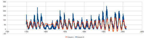
Fig. 3. Power spectrum analysis of the monthly average sunspot number record. (A) We use the multi-taper method (MTM) (solid) and the maximum entropy method
(MEM) (dash) (Ghil et al., 2002). Note that the three frequency peaks that make the Schwabe sunspot cycle at about 9.98, 10.90 and 11.86 years are the three highest peaks
of the spectrum. (B) The Lomb-periodogram too reveals the existence of the same three spectral peaks.
In the main text he says:
Fig. 3 shows high resolution spectral analyses of the monthly
resolved sunspot number record from Jan/1949 to Dec/2010 for
3144 monthly data points. The multi-taper method (MTM) (solid
line) indicates that the sunspot number record presents a wide
Schwabe peak with a period spanning approximately from 9 to 13
years, as seen in the solar cycle length probability distribution
depicted in Fig. 2. The second analysis uses the maximum entropy
method (MEM) (Press et al., 1992). The third analysis uses the
traditional Lomb-periodogram, which further confirms the results
obtained with MEM. We use MEM with the highest allowed pole
order, which is half of the length of the record (1572 poles): see
Courtillot et al. (1977) and Scafetta (in press) for extended discus-
sions about how to use MEM.
Some time ago, Bart had a thread here which went into detail on Power Spectral Density analysis:
In it we find this:
“The PSD of this is the Fourier transform of a constant R(0)^2 plus the scaled convolution in the frequency domain of the Fourier transform of R(t) (PSD of the underlying process) with itself (i.e., multiplication in the time domain results in convolution in the frequency domain, and vice versa).
The sunspot count appears to reflect the energy of these combined processes at around 20 and 23.6 years, which necessarily has apparent periods of 0.5*T1, 0.5*T2, T1*T2/(T2+T1), and T1*T2/(T2-T1) years, or 10 years, 11.8 years, 10.8 years, and 131 years. This latter appears as a quasi-beat period in the data. I say “quasi-” because these are not rigidly defined periods of steady state sinusoids, but mean periods of random excitation of resonance phenomena.
It is pretty clear that the model for the process governing Sun spot occurrence is the correct one, even if the parameterization is somewhat statistically uncertain…
When I asked Bart if this uncertainty might mean that the values could actually be 9.93 and 11.86 the reply I got was “Sure they could”. That led me to write my Jupiter Jackpot article:
Which pretty much covered the same ground as Scafetta’s analysis has now done wrt to these quantities, plus a few extra points of corroborating circumstantial evidence for Jupiter and Saturn being important players in modulating solar cycles.
Tell us more about which spectral analysis method you chose and why. I’m interested in the 10.59 year ‘lump’ which shows up in your spectral analysis and periodogram. You said:
“The omitted item is larger than the included 11.8y”
I assume this lump is what that statement refers to, but how did you get to the ‘correct value’ of 10.47 years?
I ask because there is a planetary frequency involved in the J-E-V cycle of around 10.38 years, and I’m wondering if that might be related.
Please enlighten me.
tallbloke says:
March 23, 2012 at 10:58 am
“Please enlighten me.”
This needs some clarification of theory. Read slowly, am writing this off the top of my head so it might contain mistakes. A lot of texts both on the Internet and in books are wrong or incomplete.
I’m showing the same DFT result (discrete fourier transform) as the paper, no problem but there will be disagreements about windowing etc. which is about suppressing artefacts which are phantoms. (not explained here)
Given the number of data samples, the period being examined in relation to the former, we are exceeding the theoretic limit of DFT on resolution of different frequencies. Might be 10 jammed together but will appear as one or a fat one spread across several (sometimes called broadening).
Unfortunately one bin might represent all periods (1/frequency) between 4 and 5 years, a fact of life unless there is longer data. (other techniques exist, fiercely complex topic)
The result of a DFT (or DFFT, DFT is identical, the extra F (fast) is purely a maths optimisation matter for computers which avoids duplicating computations), because it is D (discrete, sampled data), contains N/2 (N is number of data samples) possible output frequencies. The width in frequency of each output value (each output is called a bin, as in waste bin) is fixed, a result of N and the sample rate.
A row of bins and the DFT sorts the data by frequency. The output is usually complex (XY vector) and therefore the real amplitude is RMS of the pair (Pythagoras) and the angular phase (atan2(i/r) are also given if not very accurately (long story includes the infamous phase wrap problem).
This means that a value in a bin means a frequency between bin centre frequency and the bin limits, but in practice it spreads more, you get a hump.
If there is a single frequency some degree of refinement can be done by interpolation because adjacent bins are non-zero, spreading. Done well this works reasonably well. An example is a electronic stringed instrument tuning tool where the sound cannot practically (*) be resolved closely enough but interpolation largely solves this.
* A handheld device computing a realtime say million point DFFT is slow and expensive, compromises everywhere.
That describes what the paper uses if without some detail.
How can I do better than the theoretic limit?
This involves relaxing purity and using heuristics.
A computer produces a principle component FT from D input data.
This is a feedback process in an heuristic loop which adjusts each Fourier component minimising some merit function, usually least squares. The test is between the input dataset and the being created set of Fourier components.
There are no bins in the usual sense, frequency resolution is infinite. Similarly phase and amplitude are accurate, within the usual math errors etc. It is very much a compromise where usually a few frequencies are sufficient for the intended purpose. A lot of explanation is omitted here.
The software took a couple of minutes to find the 5 items requested, as far as it was concerned entirely on automatic defaults those were the most important.
As usual with heuristics, a long interest of mine, the human brain is involved, if only as a sanity check on the result. A good example is the TSP (travelling salesman problem **) which is infamous in teaching computer science and in having very real application. This is a known impossible to computer problem *in a reasonable time* for real instances. The only correct answer is via exhaustive search, which mushrooms like n! with size of problem. There are heuristic methods which can give a good answer but not necessarily the actual correct answer. This is considered good enough for real work. A human ought to keep an eye on the result and know it might be wrong.
In addition involved here is a simple technique, I like simple. Transforms (many kinds) are reciprocal so there are IDFT, IDFFT, IFT and so on, where I is inverse, backwards. Given data in the frequency domain, turn it back into a time series.
If you take a time series, DFFT and then IDFFT, and subtract the output from the original… you get a straight line of zero, within math errors.
Slow reading
Now, if I subtract those periods transformed from the SSN dataset the result is whatever is in the data without whatever those frequencies do. Now, if I do a DFFT on the result and plot it those frequencies are notched out, missing. See the plot I showed earlier, which might not have made sense… if it does now anyway. Now you know what the XLS is too. (add your own copy of sidc ssn monthly and you have the stuff to recreate the dataset used for the notched out spectra I showed above), just subtract from the dataset month by month. (nothing complicated here, all trivial by intent)
If the paper had shown the “after” spectra the problem would show.
That will do. Rog asked a short question… and ran away.
Questions? No problem.
** TVP. You have to drive to a customer in every town in England, what is the shortest distance, ie. the order you visit them? Classic network mesh stuff, edges and vertices. Min/max cost. Hugely wide applicability. (probably inside GPS nav. software too)
The WUWT thread on Scafetta’s paper has been re-opened
Martin Lewitt says:
March 23, 2012 at 9:11 pm
A scientific work doesn’t have to be falsifiable to be scientific or legitimately publishable under peer review. It can be a report of observations. Or it can be a meta-theory that while not directly falsifiable itself, generates falsifiable hypotheses.
This Scafetta paper is an observation of a statistical fit between some calculations and some data/observations. The calculations, data, statistical inferences or the strength of the statistical inferences can be wrong. But they can be right without justifying all this fuss. Despite the planetary inspiration of the calculations, the hypothesized “link” to solar and climatic variation may ultimately found to be spurious. Future data, the next couple of cycles, may weaken the statistical link. Other periods within the solar system or a better understood solar dynamo may be shown to have a better statistical fit. A more physically based model may confirm the link or show how the such periods of statistical fit can occur yet be spurious.
The physical plausibility of an actual link is better supported by general relativity of extended bodies than by newtonian tides, although the scaling factors are the same, the masses and cubes of the distances. The quadrupole moments of the solar system, the sun, and the yet to be fleshed out extended internal structure of the solar dynamo are all details to be eventually considered. The relatively much weaker role of Saturn may separately turn out to be spurious and replaced by other statistical links and a better understanding of the dynamo/jupiter interactions.
The more massive exo-planets that Svalgaard proposes as counter examples may lack the relationship between orbital and dynamo periods that make coupling of the oscillators given well established examples involving far less wrenching forces. The orbital periods are all an order of magnitude shorter than that of our most familiar stellar dynamo. So the lack of confirmation outside the solar system given the short history and questionable comparability of the examples is hardly a refutation.
From Svalgaard’s slides, I can’t tell how the rotation and revolution descriptions were used. However, from past interactions and the use of the words “free fall”, I know that Svalgaard did not seem to appreciate (few do) the extended body implications of general relativity, that can be approximated by quadrupole and higher moments. However, the conceptual difference from newtonian gravity is easy to appreciate in a dynamic system, just with consideration of the implications of gravity propagating at the speed of light (or less) rather than being an instantanous field. Different components of an extended body will experience accelerations from self-structure and external bodies at different directions and points in time.
Scafettas paper remains an observation and related hypotheses. Ideally, at some point in the future we will have a model of the solar dynamo with convincing intrinsic periodicity and incorporating relativistic planetary influences (or at least gravity propagating at the speed of light) that either confirms of refutes the relationship.
tallbloke says:
March 24, 2012 at 2:53 am
Bart says:
March 24, 2012 at 1:37 am
Willis Eschenbach says:
March 21, 2012 at 10:19 am
“…you can still claim that the parameters have some real-world basis because they are supposedly “closely related” to one of the literally hundreds of possible astronomical cycles.”
This is a valid criticism. Given the full set of astronomical cycles, it is not unlikely that you can find some which are close to those which, when arbitrarily combined, can reproduce whatever cyclic behavior you are trying to reproduce.
Most of the people who are developing the theory are not so naive as to latch onto just any combination of planetary periods which happen to match the solar and terrestrial cycles observed in proxy records and the instrumental records. Logical considerations related to the theoretical ‘power’ of the several possible physical mechanisms (tides, other types of spin orbit coupling, electromagnetic feedback) inform decisions about the relative likelihood of the effectiveness of different planet’s possible contributions. This ‘narrows the field’ considerably.
In this paper, Nicola Scafetta considers the solar system’s two biggest planets, Jupiter and Saturn. You found periodicities in sunspot data which independently led to the identification of periods which closely match those of these two planet’s interaction.
Which then led to my article:
Schwentek and Elling, back in 1984 observed that
“The clearly dominant spectral band in sunspot number, the solar cycle of 10.8 years. is given by the configuration period of Jupiter and Saturn (19.859 yr) times the ratio of their distances from the Sun (0.545)”
Further proof that the orbital distances and periods are intimately linked with fundamental solar quantities is given by the fact that :
Orbital Period (Earth) 1 year
————————————————- = Average Spin Rate (Sun) 0.0843 years = 30.79 days
Orbital Period (Jupiter) 11.86 years
There also seems to be a relationship between the period of conjunction and opposition of Jupiter and Saturn (half the synodic period), Earth’s orbital period and the solar rotation rate near the solar poles.
1 year
—————- = 0.1 years = 36.78 days
9.93 years
Furthermore, the Solar equatorial rotation rate is given by
3* Earth orbital period
___________________________ = 0.07 years = 24.5 days
2* Jupiter – Saturn Synodic period
Given these intimate relationships, it seems obvious to me that the relationships you would expect to develop in the formation of the solar system have been maintained as it has evolved.
That requires feedback. That means the solar system really is a system.
I haven’t read the comments on either WUWT or this blog regarding your paper.
I have a problem with equation (3).
The purpose of equation (3) is to relate the synodic period of an observation to its sidereal period.
Also, there’s a sign change depending on where the planet is an inner or outer planet based on the planet where you’re making the observation.
Rewriting (3) (ignoring the adhoc insertion of 1/2) as
1/P_JS = 1/P_S – 1/P_J
and noting since we know sidereal times for Jupiter and Saturn, then the only unknown is the synodic period of Jupiter when viewed from Saturn.
Since Jupiter is an inner planet relative to Saturn, the sign in the equation needs to change, hence
1/P_JS = 1/P_S + 1/P_J
which yields.
P_J = 8.34 years (synodic)(see followup comment by author)P_J = 19.82 years (synodic)
as the synodic period of Jupiter as viewed from Saturn.
And since your paper relies on the frequencies derived from the power spectrum of the sunspot data (using maximum entropy to locate the frequencies), I’m puzzled as to why it was even included in the paper.
Hi AA and welcome. Eq3 is calculating the tidal forces on the Sun, and so the periods given are the sidereal periods wrt the Sun. The insertion of the 1/2 in the equation calculating the synodic period is not ad hoc. It is there because the half synodic period is also tidally effective. That’s why 9,93 shows up in the spectrum of the sunspot data.
The same basic sscenario is laid out in the article I wrote last year
Hope that helps.
Agile Aspect says:
March 24, 2012 at 10:51 pm
P_J = 8.34 years (synodic)
as the synodic period of Jupiter as viewed from Saturn.
;———————————-
Opps – I copied the wrong number.
I should have wrote:
P_J = 19.82 years (synodic)
But this is the synodic period of Jupiter observed from Saturn so I’m confused as to why it’s included in a paper on sun spots.
Well, because it’s also the synodic period of J&S as seen from the Sun. 19.86 years
Synodic conjunction is a heliocentric alignment.
19.86 is also very close to the primary gravitational force acting on the sun, vector sum of planet forces. I say close because this is an ambiguous area. Bit of a chicken and egg.
tallbloke says:
March 24, 2012 at 11:28 pm
Well, because it’s also the synodic period of J&S as seen from the Sun. 19.86 years
Synodic conjunction is a heliocentric alignment.
;——————————————————–
19.86 years is the synodic time period for Saturn, i.e., while standing on Saturn looking inward toward the Sun and then noting the time period between Jupiter alignments.
It also says nothing about the inclination relative to the elliptic plane or anything about the orbit.
See
http://astronomyonline.org/Science/SiderealSynodicPeriod.asp?Cate=Home&SubCate=MP01&SubCate2=MP040203
Tim, interesting comment. I’m uncertain what you mean by ‘primary gravitational force’ so tell us more!
AA: “It also says nothing about the inclination relative to the elliptic plane or anything about the orbit.”
I have done some work on the ‘z’ axis perturbations of the Sun from planetary motion above and below the solar equatorial plane. All the Jovian planets are pretty close to the ‘plane of invariance’ so I’m not sure where you are going with that.
The eccentricity of Jupiter’s orbit is something the late Timo Niroma was interested in, google his stuff on the relationship between Jupiter perihelion and solar activity.
About the dominant gravitational force, the vector sum of all the forces.
Doesn’t really matter what you look at, are all roughly the same and this is what came to hand, note I am playing with in development software (not mine) which has problems, hence the plots are scruffy.
The point here is if this doesn’t show in sunspot data, smaller amplitude components stand very little chance.
(dataset, computed from ephemeris, daily data 1749 – 2047)
tallbloke says:
March 26, 2012 at 1:00 am
Bart says:
March 25, 2012 at 10:45 pm
Rog – There are a lot of coincidences in the universe. It’s just not enough. There has to be a causal mechanism to connect these things, and I just do not see one readily apparent. I’m as certain as I can be it isn’t gravity or the apparent motion of the Sun relative to the planets.
You may be right. In which case we’ll need to have a rethink about the microstructure and macrostructure of space, because as I see it, there is no way the solar system can be stitched together the way it is, shot through with harmonics which persist in time, if there is no causal mechanism linking them. If it’s not gravity or electromagnetism via the void, then the void isn’t as void as we thought it was.
Whatever is causing the ~60 year cyclic or quasi-cyclic variation in the GATM, it is there. That is the major thing right now. Determining its origin may take decades of additional research. But, right now, it is readily apparent in the data. Within the next decade, it will become undeniable. And, that means that the anthropogenic impact on the climate, at least through release of long sequestered CO2, is negligible. That’s my opinion, FWIW.
The ~60 year cycle may persist, although not as strongly as in the late C19th and C20th, due to the destructive interference of other oceanic oscillations besided the PDO and AMO, and the now out of phase ~75 year Lunar and underlying 45 year solar system signature. As Willis says above, there’s lots going on, and it isn’t simple to untangle.
I still prefer to build as a celestial mechanic than be a stats monkey wrench in the works, though we all have a role to play. Checks on enthusiasm balance the overly-optimistic resistance against chaos. Some chaos is inevitable, but a large part of what is believed to be chaotic is the interaction of cycles we haven’t disentangled yet because we gave up and didn’t try hard enough.
I think Nicola Scafetta’s model will be vindicated in the long run, but it won’t be in our lifetimes, as we haven’t yet achieved the integrated understanding of the relative power of the various strong cyclicities well enough to predict at a timescale short enough to be of real value and interest to human society, which really needs decadal scale weather knowledge at regional resolution.
I still think we’re headed in the right direction though, and who knows, another breakthrough may be just around the corner.
Cheers
TB
tallbloke says:
March 26, 2012 at 9:03 am
“…as we haven’t yet achieved the integrated understanding of the relative power of the various strong cyclicities well enough to predict at a timescale short enough to be of real value and interest to human society, which really needs decadal scale weather knowledge at regional resolution.”
Predicting the solar signal needs to be at a monthly scale and less to be useful for weather forecasting, and this is not done by integrating cycles, but by understanding the heliocentric angular relationships that are the cause of all the short term deviations.
Hi Ulric, do you have any specific forecasts linked to any specific angular relationships for this summer in mind?
I think the 10.895yr average period, and the 61, 112 and 133yr beat periods are meaningless as they do not coincide with the real Jupiter perihelion`s and Jupiter/Saturn syzygies. The precession of Jupiter/Saturn syzygies is initially 794yrs (40 synods), though every third one needs to be 43 synods to correct a slip, so much less than the claimed 983yrs.
If oppositions and conjunctions of Jupiter and Saturn are considered to result in an equal tidal force, then the oppositions in 1911 and 1970 should have had some positive effect which is very at odds with those points being the lows of c.60yr cycles.
The last time the Jupiter/Saturn conjunct`s were closest to Jupiter perihelion was in 1702 and 1762, which is problem as it was much warmer bang in between these dates.
Ulric, I agree with point one, and that’s why the solar cycles are rarely 11 years, but cluster near 10.4 and 11.9 years. But that doesn’t make the average meaningless, it just establishes the numerical relationships rather than assisting in specific predictions.
Point two: If every third precession cycle need three synods adding, why not just add one to each precesssion cycle?
The 983 years is close to the period Semi calculated (after he corrected his earlier figure), for the ‘cycle of angular momentum in the solar system’. What else he was including which makes the difference I’m not sure. maybe the other two gas giants make a difference here?
tallbloke says:
March 26, 2012 at 10:20 pm
“Hi Ulric, do you have any specific forecasts linked to any specific angular relationships for this summer in mind?”
More importantly, sorry to be a heretic, but from my analogues, I see a return to a generally warmer period from 2025 to 2038, which also follows a fairly long standing pattern of warmer decades centred at 1630, 1730, 1830 and 1930. Even Leif mentions a c.100yr cycle in solar activity, though curiously it does not show up in the power spectrum.
p.s. I`ll mail you about summer.
tallbloke says:
March 26, 2012 at 10:56 pm
“Ulric, I agree with point one, and that’s why the solar cycles are rarely 11 years, but cluster near 10.4 and 11.9 years. But that doesn’t make the average meaningless, it just establishes the numerical relationships rather than assisting in specific predictions.”
Averaging solar cycle length is fine, and they should cluster at 6.5 and 7.5 Earth/Venus synodic periods.
Averaging Jupiter orbit period with Ju/Sa half synods is like seeking e.g. the average between the lunar synodic period and the anomalistic month, which is pointless, when what is needed is their integer ratios, i.e. whole numbers of both of them (or very close to), and that is when they re-coincide to make a perigean tide.
“Point two: If every third precession cycle need three synods adding, why not just add one to each precession cycle?”
Because the trigon has moved round 120 degrees in that time, it takes 13 trigon`s and ONE extra synod to return them both to roughly the same location. So nearest to the start point is either at 40 synods or at 43 synods, at 41 synods they both will be c.120 deg away from where they started.
“The 983 years is close to the period Semi calculated…”
There is a good 5 body return at 953yrs that can pick a season, e.g. winters 1010 and 1963, though critical changes in Neptune`s relative position will change the phase as it is not a component of the cycle. You could say that there is roughly a 1157yr return of events, but it cannot be exact as the sequence of events will be different at each node, the first time they get particularly similar is at 4627yrs. A more accurate description would describe an event series of configurations for 2224yrs, a single 179yr step, then the mirror image of the first 2224yrs worth of configurations (in reverse order) to complete the 4627yr cycle. It won`t be quite that clean as the orbits are not circular.
Ulric, excellent input, and thanks for the email.
Very interesting.
I do not have the time or capability to study, digest and review all this material.
But I can still learn. I gather planetary motion and alignment affects Earth tides and solar radiation intensity, apparently pulling and squeezing the plasma ball, which affects Earth’s temperature cycles.
The predictive power of Scaffeta model is impressive.
One central tenet of UN IPCC GHG theory is: once all other external inputs are accounted for, it is proper to conclude residual temperature changes are caused by fossil fuel combustion production of CO2. That is not allowed by science. Because it is not possible to identify, let alone account for all external inputs. Someone like Scaffeta will come along and identify another one.
Scaffeta discovery shows why this is true. He also shows the proper approach for analyzing and quantifying cause – effect phenomena. Nothing like a good theory and data analysis. A useful standard for those still struggling to figure out the effect of fossil fuel combustion on [CO2] and any possible effect on T.
I too have noticed decline in quality at WUWT.
If I were a journalist, my headline would be: Prof Nicola Scafetta discovers an important cause of Earth’s temperature cycles is planetary motion influence on solar radiating intensity. Model fits main cycle data since 10000 BCE. He predicts low solar activity and a cooling period 2020 to 2040 for Earth.
Hi Pierre,
The effect of Jupiter and Saturn on Earth’s Moon and Sun dominated tides is immeasurably small. Some argue the effect of Jupiter and Saturn’s tidal effect on the Sun is immeasuably small too. However, the high solar surface gravity and extremely mobile plasma medium might mean that he horizontal components of that tidal force might not be negligible.
Dr Scafetta doesn’t concern himself too much with the mechanism by which the effect might be occurring, but concentrates instead on the synchronicities of the planetary motion and the solar activity levels.
From the paper:
“A simplified harmonic constituent model based on the above
two planetary tidal frequencies and on the exact dates of Jupiter and Saturn planetary tidal phases, plus a theoretically deduced 10.87-year central cycle reveals complex quasi-period interference/beat
patterns.The major beat periods occur at about 115, 61 and 130 years, plus a quasi-millennial large
beat cycle around 983 years.”
1) There is no central cycle, it does not exist as a cycle.
2) The clustering of the solar cycle lengths at 10.39yrs and 11.99yrs is exactly what would be expected from the alternate superior and inferior conjunctions of Earth and Venus in line with Jupiter through each cycle maximum (and solar magnetic reversal). The configurations alternate at each cycle, which means the cycles follow a pattern of 6.5 Ea/Ve synods in one cycle, followed by 7.5 synods in the next cycle. Hence there is no need to perceive these periods as “side attractors”, or anything to do with Saturn at all.
3) Regarding fig 4 {A} in the paper, tighter Ju/Ea/Ve heliocentric stelliums (all three in line on the same side of the Sun) appear at the frequencies: ~65.5yrs, ~89.5yrs, 110/113yrs, and 131/134yrs.
This gives a far more plausible and direct explanation for the power spectrum results.
Ulric, excellent stuff, thanks. To my way of thinking, the fact that both the JEV cycles and the average JS timings coincide with the relevant frequencies is just more grist to the planetary mill.
The long term average synodic period of Ju&Sa multiplied by the ratio of those two planet’s distance from the Sun = 10.8. The Sun is in the long game as well as the short one. Stability and variability.
tallbloke says:
March 30, 2012 at 10:54 pm
There is no sane reason to take an average of the 9.93yr and 11.86yr periods.
Now if 115yrs or 130yrs would divide by 9.93yrs or 11.86yrs, but they don`t, so they have nothing to do with Jupiter sidereal period or Ju/Sa spring tide.
“There is no sane reason to take an average of the 9.93yr and 11.86yr periods.”
The deviations from the average values of the two periods produce a coherent pattern which is seen in data representing the alignment along the parker spiral.
tallbloke says:
March 31, 2012 at 10:05 pm
“The deviations from the average values of the two periods produce a coherent pattern which is seen in data representing the alignment along the parker spiral.”
Nicola is talking about tidal forces, they can`t act along spirals. It is not clear what you mean by “The deviations from the average values of the two periods..” ?
[…] on this blog here. At WUWT […]
[…] on this blog here. At WUWT […]
[…] Nicola Scafetta also created a long term reconstruction using planetary periodicities in his paper : […]
[…] on Jupiter and Saturn’s relationship with the solar cycle and independently confirmed by Scafetta 2012a[7] are […]