


Guest post from Andrew Cooper, AKA ‘Scute’. It’s a bit hard to tell if the baseline for temperature on video version from the IPCC press conference runs from 1861 or 1851, so we’ll let the talkshop readership decide. They certainly did switch the cumulative emissions baseline. It all makes a difference to presentational impact, especially the misleading slope in temperature from 2000-2010.
graph from page 36 of the Summary for Policy Makers (SPM) with the version shown at the IPCC press conference below :
http://www.climatechange2013.org/images/uploads/WGIAR5-SPM_Approved27Sep2013.pdf
The graph includes an unabashed cherry-picking of temperature data points (2000, low and 2010, high) so as to fit the linear relationship the IPCC are promulgating between total accumulated CO2 and temperature since the late 19th century. It is true they can say they were just plotting in tens of years, to show a long term trend from 1860 but the current 15-year standstill is now turned into a soaring rise. They, of course, know this is a complete misrepresentation of the truth but are hiding behind the fig leaf argument that the decimal system dictates that you choose years with a ’0′ on the end.
This is made worse by the fact that the graph was touted in the live streaming of the SPM press presentation but is languishing on the last page of the 36-page SPM document. And you had to be quick to see the problem in the few seconds that they zoomed in on it at the conference.
Here is a clip from the BBC where they parade the offending graph (at 1:30):
http://www.bbc.co.uk/news/science-environment-24292615
Notice that Thomas Stocker, the co-chair of Working Group 1, says it was finalised “after many hours of deliberation and preparation by the scientists”.
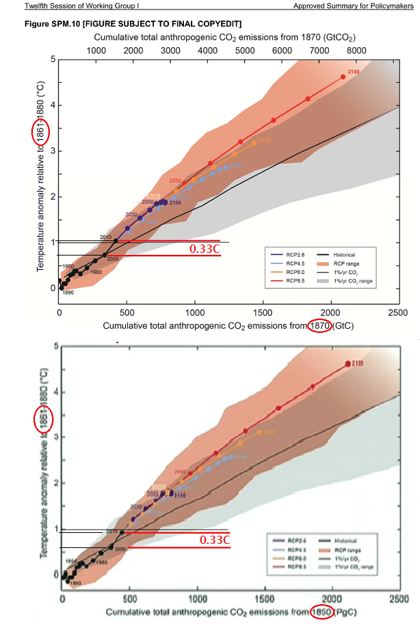
There is so much wrong with this graph. For a start, there are in fact two versions, one presented at the conference and the other on page 36 of the SPM. You can tell because the 2010 temperature plot is at 0.91 C (above 1861 to 1880 average) in the press conference graph and at 1.05 C in the printed summary. The 2000 temperature has crept up between the press conference video and the print version too. It’s at 0.59 C in the video and at 0.74 C in the print version. That’s a 0.14-0.15 C discrepancy between two sets of historical (i.e. set in stone) data. The 1861-1880 baseline is the same for both graphs so the plots should be identical. The same thing is happening to the 1950 and 1980 plots.
In other words, the “preparation” done by the scientists was to take the page 36 SPM print version and shunt the entire historical plot down by 0.15 C- that’s a decade’s worth of warming. No wonder they “deliberated” for “many hours” over it and got not a wink of sleep. The video version of the plot now sits a little lower and seems to show off the linear trend rather better. So they probably think their lucubrations paid off. Trouble is, in their haste they allowed two incompatible graphs to slip into the public domain.
It doesn’t end there. According to the 3 main temperature sets, averaged, there is a 0.253C difference between the 2000 and 2010 temperatures. Both the offending graphs show this difference to be 0.33 C. The combined datasets show around that trend from 1990 rather than from 2000!

The cherry-picking of these two dates is already a gross misrepresentation of the underlying data but the spurious stretching of the gap allows an even steeper upward kick where, as we know, there is a flatline. If that flatline had been shown, it would have drifted off horizontally to the right with never a hope of linking smoothly to the projected future trend that soars above it. An ugly 90 degree vertical hike would have been unthinkable so, indeed, “much deliberation” was needed to devise a way of avoiding it.
Source for global averaged temperature: Hadley Centre Global Temperature page (table at bottom).
http://www.metoffice.gov.uk/research/monitoring/climate/surface-temperature
Deliberation’ and ‘preparation’. Those two words sound like euphemisms for something rather stronger. Stocker uses them specifically and exclusively in relation to this graph.
This all smacks of massaging the plot data to fit a dubious narrative (force-fitting the linear trend emphasised in the video) and soaring temperatures (plus ca change). I think Thomas Stocker and his scientists should be called on it.
APPENDIX
There is one legitimate difference between the two graphs. The press conference graph shows cumulative carbon emissions from 1850; the print version shows it from 1870. This difference shunts the plot along the x axis by a tiny amount for the press conference version. This has no bearing on the spurious shunt of the plot down the y axis for the temperature. As stated above, both graphs cite the 1861-1880 baseline.
The temperatures were measured carefully with a ruler with the plot zoomed. They are the most accurate readings I could get. I concede that they could be out by 0.02 to 0.03deg C. However, this is a small fraction of the discrepancies discussed and therefore doesn’t detract from the thrust of the article.

There is always the possibility I am not reading the graphs properly, but the cumulative CO2 graph surprises me. The graph of emissions on the US EPA website shows that emissions have accelerated in the second half of the 20th century.
http://www.epa.gov/climatechange/ghgemissions/global.html
Steve McIntyre has commented on similar lines. He concludes:
‘the earlier projections have been shifted downwards relative to observations, so that the observations are now within the earlier projection envelopes. You can see this relatively clearly with the Second Assessment Report envelope: compare the two versions. At present, I have no idea how they purport to justify this.’
If sleight-of-hand tricks are needed to make your case, you haven’t got much of a case.
This post motivated me to go through the IPCC’s SPM figures, and having now done so I have to say that the IPCC has done an excellent job of hiding the skeletons and papering over the cracks. To someone who is unaware of the numerous problems with the AGW hypothesis, or who chooses to ignore them, these figures make a visually compelling case that AGW is still alive and well.
The key figure is the second graph on Figure SPM.1 (a), link below, which gets around the problem of the warming “pause”, or “hiatus”, or whatever you want to call it (personally I like “apogee”) simply by plotting decadal rather than annual means. If you wanted to convince a friend that the earth was still warming this graph is probably all you would need. But if it wasn’t enough you could add the later SPM Figures, which show everything moving in the direction AGW says it should – temperatures, CO2, sea levels, ocean heat content etc. increasing and ocean pH, snow cover and Arctic summer ice (gone by 2081, by the way) decreasing. Even the model-observed temperature comparisons in Figure SPM.6 show good fits – a remarkable result given that most of them are regional comparisons and even the IPCC admits that climate models don’t work too well at the regional level.
As for Figure SPM.10, if you were a bureaucrat or a politician wanting to be reassured that you still had a job or that your emissions-cutting policies were still 97% supported by the science you probably would have put down the SPM draft before you even got to it, breathed a sigh of relief and poured yourself a scotch. But had you looked at it your initial reaction would have been; what’s this? And assuming you were able to figure out what it was you would find that the problem with it isn’t so much the cherry-picked years as the fact that observations and projections aren’t segregated. Both are plotted as solid black, orange, blue or red lines extending all the way from 1870 to 2100. But at that point you don’t care. You just pour yourself another scotch.
What I don’t get is how they can have a different trend for each 10 year period and have them all join up neatly. See what I mean here:
http://woodfortrees.org/plot/wti/from:1980/to:1990/trend/plot/wti/to/plot/wti/from:1990/to:2000/trend/plot/wti/from:2000/to:2010/trend
Also, that shows a much higher trend 1990-2000 than 2000-2010. What data are they using?
I used the wti 4 main indices average.
You only have to shift the endpoints of the periods a couple of years to see the serious issue with non-matching endpoints.
http://woodfortrees.org/plot/wti/from:1980/to:1987/trend/plot/wti/to/plot/wti/from:1987/to:1997/trend/plot/wti/from:1997/trend
Are they really expecting us to believe endpoints match for every decade back to 1850. Some serious numpetry going on here.
TB: Your graph shows TLT. The IPCC uses three “combined land + ocean” surface temperature data sets – probably HadCRUT4, GISS LOTI and NCDC land & ocean.
And the shifts on your second graph coincide with ENSO events. 🙂
I cannot understand the significance of the cumulative anthropogenic CO2 emissions – is it assumed that there is no increase in CO2 absorption or sequestration – say as dissolved in rain falling into oceans? I always had it in mind that this was a homeostatic system?
A cynic might say that whatever the IPCC comes up with can be summarised thus:
‘Well they would say that wouldn’t they?”
(From Andrew Cooper)
Rog
Thanks for measuring the jump between 2000 and 2010 as 0.33 C. I made it 0.32 but stuck with “over 0.3”. I think that the 0.07 discrepancy (.25 to .33) is what they absolutely cannot justify because it’s independent of whatever baseline is used. It should be .25, as averaged from the 3 main data sets that Roger Andrews cited. There’s a lot of smoke and mirrors with these graphs but that discrepancy is a numerological inexactitude is it not? Regarding all the other stuff they can keep swopping fig leaves but they should have their feet held to the fire on this one point.
As for the 1850/1860 question for the temperature baseline in the video, I see what you mean. Zooming in on my screenshot of the video, there is a hump at the top which suggests a ‘6’ but a sharp turn on the upper-left inside edge, suggesting a ‘5’. But the ‘8’s have flat undersides to their curved tops. It’s a difficult one, but one clue to it being 1861 is that Thomas Stocker refers to that axis as the temperature of “the late 19th century”. I suppose 1850-80 is late too, but I wouldn’t readily call it that. I would say “mid- to late”.
Andrew
Roger A: “And the shifts on your second graph coincide with ENSO events.”
And they never happen at the ends of decades?
” Your graph shows TLT”
UAH and RSS TLT combined with surface T from HADcru and GISS.
Andy: Maybe the best way to tell is to see what difference the 10 year shift in baseline makes. If it finds the same ~0.15C difference, then there it is.
As for the 0.33C trend they’ve stuck on there, it’s wrong. End of.
Going back to my wti plot, the slope for the 90’s is way bigger than that for the 2000’s. Lets see what HADcru variance adjusted global says:
http://woodfortrees.org/plot/hadcrut3vgl/from:1980/to:1990/trend/plot/hadcrut3vgl/from:1979/plot/hadcrut3vgl/from:1990/to:2000/trend/plot/hadcrut3vgl/from:2000/to:2010/trend/plot/hadcrut3vgl/from:2010/trend
Yup, still bigger.
Hmm, this is interesting: here is a wft comparison of 1851-80 and 1861-80. If you take the average of each of these two lines you get something like a 0.15 degree difference but when applied to the two graphs it’s shunting the plots the wrong way!
http://woodfortrees.org/plot/hadcrut3vgl/from:1851/to:1880/trend/plot/hadcrut3vgl/from:1861/to:1880/trend
confusingly for us, the temp scale on this wft graph is referred to the 1961-90 baseline but that is immaterial because we are looking at the absolute difference in two temperatures, between the two averaged lines. Those two temperatures would then form the baselines for the 2 IPCC graphs (assuming the video graph really does say 1851-80)
Please correct me if I’m wrong but to get the baseline average it seems intuitively correct to measure the length of the line and then strike off horizontally to the temp scale from the midpoint of that line, yes? I know wft probably has a tool for it.
Anyway, by adopting that method, I come up with about -0.32 C for 1861-80 and -0.335ish for 1851-80.
Now, you might think, ‘there it is, that’s the 0.15 C increase in the plot between the video and the print version so the video must have an 1850-80 baseline, not 1860’. But if that were the case, the video plot should be higher than the print by 0.15 C, not lower! Since the baseline is 0.15 degrees lower, there should be a bigger difference between that baseline and the 2000/2010 temp readings. But the video version is just below 1C (0.91) and the print version is higher (1.05).
However, it seems too much of a coincidence that I’ve found a 0.15 C difference using wft. Could it be that they saw the difference and applied it the wrong way round?
This assumes it really does say ‘1850’ on the video version of the graph. My screenshot is clearer but still difficult to discern.
Andrew
The debate rumbles on, here:
http://skepticalscience.com/ipcc-model-gw-projections-done-better-than-you-think.html#.UkpVR8JIOhg.twitter
One commenter notes:
“A projection is not making a prediction or forecast about what is going to happen, it is indicating what would happen if the assumptions which underpin the projection actually occur.”
But why make assumptions in the first place?
Roger and Andrew,
some of the concern expressed here seems linked to the assumption that the black line on this figure (Fig. SPM.10) represents observations and thus should match the HadCRUT4+GISS+etc. data. This isn’t the case. Fig. SPM.10 is based solely on simulations from models, as stated in its caption on page SPM.20. For the black line:
“Model results over the historical period (1860–2010) are indicated in black.”
So the black line is the mean of multiple simulations with multiple models, all forced by estimates of the historical sequence of forcings. This is why the black line doesn’t have the features you are expecting, related to the recent slowdown in surface warming, the exact offset between different decades, etc.
The caption also says:
“Some decadal means are indicated for clarity (e.g., 2050 indicating the decade 2041−2050).”
So these are decadal means, not simply individual years picked because they end in zero. The point labelled “2000” is thus the mean of 1991-2000 from these model simulations.
Hope that’s useful
Tim
OB can’t help myself but the IPCC have made an ass [of] u [&] me 🙂
I have been wondering, since it is clearly a political excercise in damage limitation I am disappointed they did not opt for 110% confidence. All we need now is a few ‘erm’s in the statements…”erm the models say it’s worse than we thought but erm we’re 110% that the erm known unknowns and erm unknown unknowns are all our fault…erm…look at this graph…”
Are the IPCC like Newcastle under Keegan – all attack & no defence? 🙂
Tim Osborne: welcome to the Talkshop, and thanks for your comment. Do you think the reason the models show a lower trend for the ’90’s than the 2000’s is primarily because of the parameter used for the volcanic forcing? Or because the downwelling energy from the increasing co2 switched to warming the deep ocean instead of the surface? If the latter, what is the mechanism envisaged by climate scientists for the passage of energy through the upper ocean?
I don’t much wonder they are doing the tricks with the graphs, that’s old vest. But where on Earth they want to get all that carbon needed to continue the interpolated trend to the 2100 is real mystery to me. Do they have couple of fresh new Saudi Arabias somewhere in hidden?
The Hockeyschtick puts it in a nutshell:
‘If you can’t explain the ‘pause’, you can’t explain the cause…’
http://hockeyschtick.blogspot.co.uk/2013/09/wsj-one-lesson-of-ipcc-report-is-its.html
Not pulling punches it goes on to say:
‘climate alarmists…use the flimsy intellectual scaffolding of the IPCC report to justify killing the U.S. coal industry and the Keystone XL pipeline, banning natural gas drilling, imposing costly efficiency requirements for automobiles, light bulbs, washing machines and refrigerators, and using scarce resources to subsidize technologies that even after decades can’t compete on their own in the marketplace.’
Not to mention trying to price citizens out of the energy market whose infrastructure they helped pay for in the first place. How much more do they expect people to take?
@ Tim Osborn October, 2nd 2013, 11:24
Thanks for that clarification, Tim. It answers a few questions for sure. It also raises a few which I’ll list below. You may be able to shed light but they are for anyone in the know:
1) The legend on the graph SPM.10 says “historical” for the black, dotted line. ‘Historical’ usually means of or concerning history or past events or simply belonging to the past. The usual understanding is that it is referring to real events or actual recorded events or data. It is quite rare that it is used for fabricated events or data such as a historical novel or film and if these bear any relationship to real past events, the extent to which they do is usually clarified from the start. Neglecting to do so gives rise to much confusion, such as a generation of kids growing up to think that the US captured the Enigma machine. Now a generation of adults think the world warmed faster in the last decade than it ever has since records began. Thomas Stocker could have cleared that up with one short sentence: “historical in this context means a hindcast of model runs”.
And that is the correct label for the black dotted line: ‘hindcast’. If the models have hijacked the meaning of the word, historical, which word are we supposed to assign to honest-to-goodness real, factual historical records? Historical might mean hindcast in IPCC parlance but not in the parlance of the rest of the English-speaking world.
2) number (1) is compounded by having the caption for SPM.10 sixteen pages before the graph it relates to. I know the copy editing isn’t finalised but why publish it at all if that same (sorry, slightly different) graph is paraded to the world and hoardes of people with any knowledge about the temperature record are going to go to the print version to query it? When they arrive, they find no caption except the title and the labelled axes and naturally surmise that those must be enough to interpret the graph. They would then, understandably, see the dated dots as dates and not decades and query it further. They would have no inkling that they could be decadal averages and no way of finding out without reading the entire SPM and stumbling over the caption for the graph after 20 pages and 16 pages before the graph itself. Meanwhile, those back at the press conference would also see the dots-as-dates leaping ever-higher but with no knowledge of the current 13-year halt in temps, they would be totally duped by a known discrepancy with reality, generated by a model hindcast showing a break-neck 0.33 C/ decade rise. I think that’s nothing short of atrocious.
3) how is it that the ‘historical’ plot mimics the real historical record (as far as one can tell from the size) but then becomes bland, straight lines after 2010? If they are models and they are plotting future trends, you would expect one of two scenarios:
a) the plot after 2010 shows all the same variability, natural or otherwise, that is depicted in the ‘historical’ portion of the plot.
b) since the models are blind to the future from their start date in 1860, not just the post 2010 portion, shouldn’t they exhibit the same bland, straight line as they do after 2010?
4) notwithstanding the point made above about the ‘historical’ plot mimicking the real historical record, why is it that the only place where it veers erratically from that behaviour is between 2000 and 2010? Bang in the middle of the 16-year pause?
5) if the points above haven’t driven it home yet, why didn’t Stocker or one of his scientists just stop and say, “wait, we at the IPCC might know that there is a) not one jot of real-world data here b) we know historical means hindcast in our parlance c) we know there’s a 0.33 jump where temps are flat and that’s OK because the model says it’s OK d) we know the dated dots are decadal averages because we say they are so we, ourselves, don’t need graph labelling BUT won’t the policy makers and general public just think this is really happening in the real world?”
There’s more but it’s too late now.
Andrew
It’s very curious to me that you come up with 0.33°C from that IPCC graph. Is that the same +0.33°C that appeared in the temperature records near the end of 1997 and also, very curiously, if removed from that one month, levels the entire trend into the past (at least per some data from WFT)? To myself I can’t to help think that sudden +0.33C as Al’s poison-pill gift to humanity while he still held the power to control. Much like this: (http://www.woodfortrees.org/plot/wti/to:1997.93/plot/wti/from:1997.93/offset:-0.33) but before I downloaded the entire dataset into a spreadsheet and removed from the the trailing so a contiguous linear regression could be also overlaid. Lost it somewhere. Well, that is probably nothing, just some artifact stuck in my mind, yet it stays stuck there, the one single alteration that seems to levels them all.
I mean you compare that thought above to the actual ocean temperatures: http://s21.postimg.org/6h0l0crzr/IPCC_Prediction_and_Ocean_Temps_L_2100.png
and I can’t help but question the data we are being asked to deal with. Remove that +0.33°C (or close) from that month and everything looks as expected.
I’d like to illustrate the point I made above (question 2) using the IPCC Summary for Policy Maker’s own data, that is, real historical data, not models. I realise the content of this comment might seem fairly obvious but it’s a case of nailing it down because it’s easy to conflate the objection to the 0.33 C rise with the misconception that the 2000 and 2010 dots are decadal means. This whole comment assumes we at the Talkshop all now know that the dots are decadal means but those at the press conference didn’t.
Part of my question 2 said:
“Meanwhile, those back at the press conference would also see the dots-as-dates leaping ever-higher but with no knowledge of the current 13-year halt in temps, they would be totally duped by a known discrepancy with reality, generated by a model hindcast showing a break-neck 0.33 C/ decade rise.”
The true decadal averages, and therefore the real-world increase from the 90’s to the 2000’s is shown in the first SPM graph, SPM.1. It is on page 27 of the SPM and its caption is on page (ahem) 3. I’ll link the whole document (36 pps) here- it downloads in seconds:
Click to access WGIAR5-SPM_Approved27Sep2013.pdf
This graph shows an increase of .18 to .19 C, depending on which dataset (coloured bars) you measure between. This means that the SPM.10 graph (p 36, caption p 20) with the ‘dotted decades’, shows a 0.14 Cto 0.15 C overshoot for 2000-2010 in relation to 1990-2000, i.e. the 2010 dot is 0.33 C higher when it should be 0.18 C to 0.19 C higher.
Stocker and his Working Group would just say it’s because it’s a ‘historical’ model run, that is, a hindcast. The points I made in my last comment show that this is yet another fig leaf as there was no way of knowing that the entire graph is model-generated and as such, contains no real-world data. The ‘historical’ plot appears to be real and so consigns the 13-year flatline to the sceptic blogs where, in their view, it belongs.
Andrew
Wayne
That wft graph with the .33 offset is interesting. I wonder if the ‘historical’ portion of the model runs were coaxed into mimicking the real historical data, perhaps by doing Monte Carlo runs. If they could do that, they could do a few more and happen upon a 0.33 C rise from the 1990’s to the 2000’s and argue that it retains something of the behaviour of the plot, if not the trend, between 1990 and 2010.
The counterveiling argument to that proposition would normally involve pointing out that the straight lines after 2010 wouldn’t be straight but exhibit all the vagaries of natural variation, just like the ‘historical’ portion. But if that puts the kybosh on the proposition, it raises the question as to by what mechanism a blind model can show natural variation up to the present and no variation thereafter. I can’t think of any mechanism whether Monte Carlo runs are involved or not.
I am also intrigued by the 0.33 C and the 0.15 C overshoot above the real 0.18 C jump from the 90’s to the 2000’s. You may recall that the entire plot in the press conference graph was dropped by 0.15 C. Now, there was as Stocker said, “much deliberation and preparation by the scientists” over this graph. Could it be that someone objected that the 2010 plot was insupportable , even as a model data point because it would be misconstrued and asked for 0.15 C to be shaved off it? Then, instead of shaving that one data point, the whole plot was dropped by 0.15 C and no one noticed or cared? It’s certainly plausible that someone would object to the jump (Saudi Arabia and others fight their corner) and after ‘many hours of deliberation’, read heated discussion, frayed nerves and lost sleep, it would be plausible to let your brain slip or your mouse slip when selecting a line instead of a dot.
It’s just a thought. It can’t be proven but there must be a story behind that plot drop whether it’s human error or the 1850/60 baseline question or something else.
That press conference graph was probably knocked about quite a bit. Another sign of this is that the temperature scale had been squashed by a factor of 1.37 which doesn’t alter the information but changes the slope and the impression given. Admittedly that means a shallower slope but who knows what their intentions were? Tallbloke resized it for comparison purposes but it only occurred to me later that it might be bearing the scars of being batted around the room. It also showed the CO2 in petagrams, not gigatons as the print version does and plotted it from 1850, not 1870. And they dispensed with the gigatons of CO2 along the top scale that’s seen in the print version. That was shown because the bottom scale isn’t CO2, as labelled, but carbon!
Andrew
P.S. Apologies for saying data point instead of datum point. I’m one of the ‘data-as-singular’ heretics as in most cases it only has meaning when used in bulk like sugar and flour. But yes, 2000 and 2010 are datum points.
The BBC’s Paul Hudson dips his toe in the waters of climate controversy again, by calling into question aspects of the IPCC summary report.
http://www.bbc.co.uk/blogs/paulhudson/posts/The-IPCC-report-is-the-science-settled
He says that the Met Office Hadley Centre specifically excluded in one of its reports the possibility of static temperature trends for 15 years – which has as we know just happened and is on-going.
He finds it ‘disappointing’ that most of the media have ignored this – something to do with the IPCC ignoring it in the summary, perhaps. Too busy talking up their barmy confidence levels based on model results that don’t even reflect the recent past correctly.
@ tallbloke October 2, 2013 at 2:45 pm
>>>>”Do you think the reason the models show a lower trend for the ’90′s than the 2000′s is primarily because of the parameter used for the volcanic forcing?”
Since the black line connecting the black dots in this figure is an average across many individual model simulations under multiple historical forcings, it is likely that most variations due to “natural” internal variability will be averaged out (since the particular sequences of internal variation will not generally be correlated between simulations).
The same is also true for the thin black line without the dots, except that CO2 is the only forcing that changes in those simulations.
The difference between the thick and thin black lines will therefore be mostly from differences in the non-CO2 forcings, as applied to the the models. Solar, volcanic, methane and other non-CO2 well-mixed greenhouses gases, tropospheric aerosols, etc.
So, yes, the warming simulated up to 2000 may have been slower than the warming simulated up to 2010 because of the Pinatubo volcanic forcing during the 90s. But it may also be related to changes in tropospheric aerosols. Looking back at the earlier dots, there are some decadal dots that lie below the thin black line: this will also be due to the non-CO2 forcings, probably volcanic and tropospheric aerosols dominating over the warming influences of other well-mixed GHGs and solar.
[Just to be clear, I was involved in neither the construction of this figure nor in the chapter that assessed this, which is why I’m slightly unsure about some details.]
@ Scute October 3, 2013 at 1:49 am
(1) Historical does indeed refer to the history of past events — in this case the (estimated) history of past forcings. Yes, it could have said “Simulations under historical forcings”. But the caption does make it clear. And it is in section E of the SPM, titled “Future Global and Regional Climate Change”. The other figure in this section that shows “historical” values (Fig. SPM.7) is also based on model simulations. “Observations” are shown in sections B, C and D.
(2) The figure and caption will of course put placed together in the typeset version. People reading or even scanning the entire SPM would see the caption. Others would expect a caption and look for it, especially if they were writing a blog post about this particular figure 😉 They wouldn’t have to read the entire SPM and stumble over it, they could simply search for “SPM.10”.
(3) The historical part of the plot shows more variations because the (estimated) history of past forcings — particular solar and volcanic — contains multi-decadal variations. These aren’t known for the future and hence aren’t included in the RCPs (just the 11-yr solar cycle), so those are blander lines, as you note. You can still see some influence of variations in non-CO2 forcings — for example each RCP curve appears to curve down towards its end, which I’ve been told is due to methane forcing reducing and bringing the RCP projections slightly back down towards the thin black line (CO2-only simulations).
(4) See my earlier answer to Roger. The purpose of this graph isn’t an comparison between observations and models, which was covered in section D. The slowdown in warming over the last 15 years has indeed been a challenge to climate models — section D reports the conclusion that there may be, in some models, an “overestimate of the response to increasing greenhouse gas and other anthropogenic forcing” .
(5) I think (1)-(4) cover this.
Tim Osborn: Thanks for making a thorough reply to Andrew. I think it goes without saying that if there has been “in some models, an “overestimate of the response to increasing greenhouse gas and other anthropogenic forcing” “, then there has been a corresponding underestimate in the natural variation forcing, and/or unforced variation, and/or anthropogenic aerosols.
I’d be interested you have your view on which it is.
I think solar forced variation has been seriously underestimated, for a variety of reasons.
For one, mainstream climate science holds that since the amplitudes of the solar cycles have been diminishing since 1960, solar can’t be responsible for late C20th warming. This misunderstands the way thermal inertia works in the oceans. It also ignores the effect of UV on the upper atmosphere. Not all joules are the same. Raw TSI figures are a blunt instrument.
Hi Scute,
“You may recall that the entire plot in the press conference graph was dropped by 0.15 C.”
No, didn’t realize that. Who is Stocker? Many, like you, know 10 times what I know of the data records, who in agencies and IPCC did what in the past and such. My time has been spent more on the physics and radiation end with the atmosphere that I do something a bit about.
Hmm. I have to admit it does seem rather implausible on the surface except I understand one single U.S. agency holds the base temperature records (GHCN??) that every other major global temperature dataset uses or calibrates to. Could there have been some political hanky-panky back in 1997 that did the trick to guarantee this to continue into the future? Really don’t know. I guess you see why after coming across that I can’t seem to get it out of my mind. i rarely delved into temperature datasets. (Well, downloaded the BEST dataset and did some rough analyses on it when it came out, I am a programmer, couldn’t resist that much data ;))
And finding that was just a happenstance, I had a question and IIRC I was questioning just how much could the entire Earth, according to the datasets, warm or cool in one single month after seeing some month’s being rather so large they were hard to swallow. Downloaded the dataset and ran a series of pot-shot analyses and stumbled upon that one single month, makes it look like nothing has happened at all over the last five decades. All of the up and down excursions even line with the historics before that.
So, the question is, can a one single month’s huge jump upward be instantly permanent so that every month following that jump is the same in the range as before the jump? I personally don’t think so and if you notice all largest excursion levels both up and down also hiked after that date. Doesn’t seem natural, the way noisy data should look if the increase was gradual.
Scute, after digging backwards through my gigabytes of crud that I’ll probably never need or use I found what cued me long ago:
http://www.woodfortrees.org/plot/hadcrut3gl/from:1997.5/trend/offset:-0.205/plot/hadcrut3gl/from:1982/to:1997.5/trend/plot/hadcrut3gl/from:1982/to:1997.5/plot/hadcrut3gl/from:1997.5/offset:-0.205/plot/hadcrut3gl/from:1982/to:1997.5/trend/offset:0.333333/plot/hadcrut3gl/from:1982/to:1997.5/trend/offset:-0.3666666/plot/hadcrut3gl/from:1997.5/trend/offset:-0.571666/plot/hadcrut3gl/from:1997.5/trend/offset:0.128333
It’s not exactly as I remember it, but I’m older now, I thought it was in an Excel spread sheet, but that’s right, I was also trying to learn how to draw upper and lower limit bands about linear regressions and the only way to naturally join was to use that 0.33C. Memory plays real tricks on you as a year goes by (at least at my age now). That is the offset I remember, 0.33C. Just trying to stay on the up and up.
Earlier in that same day I had another with 0.34C and that may have cued me try that value and it did mesh them as expected. Look like the month number is off by a couple too.
As I said, that is curious but may be all it is.
@Tim Osborn October 4, 2013, 4:17pm.
Thanks Tim for your comprehensive reply to my questions. I appreciate your input at the Talkshop.
I’ll leave it to the contributors to asses whether your genuinely interesting description of the process provides a basis to excuse Stocker and the scientists of Working Group 1 for showing the SPM.10 graph at the press conference.
I note that you had no input on that graph or chapter and realise that you don’t profess to be an apologist for WG1 (nor need to be) so the above paragraph is a plain statement, not a tacit challenge.
As one of the contributors, here is my assessment, distilled into narrative form:
I would be absolutely delighted if I came up with a model that shadowed the real historical record from 1860 and overshot the 2000’s by only 0.15 C. What’s more, I’d probably email it to my confreres at the IPCC straight away, encrypted of course;). Being inveterate caption hunters and prolific decade-dotters themselves, they would immediately see its authoritative sweep and surely congratulate me. What I wouldn’t then do is call a press conference and flash it to a billion busy people for 30 seconds without an exhaustive explanation as to the extent to which the graph represented real history as opposed to estimated history. I would also read out the caption to clear up the dotted decades issue and drive the point home by saying “this entire graph, from 1850 to 2100 is the product of computer models, based on simulated forcings for historical as well as future projections and the black, dotted line does not represent the temperature you have been experiencing for the last 13 years.”
And if I got even halfway through visualising this unlikely scenario I’d shelve the graph and find something honest and simple to show the world.
Andrew
Wayne
Thomas Stocker is the co-chair of Working Group 1 at the IPCC. He presented the graph at the press conference, linked here (graph shown at 1:30):
http://www.bbc.co.uk/news/science-environment-24292615
Notice how Stocker brazenly refers to the vertical temperature scale as “you see on the vertical, temperature anomaly relative to the late 19th century.” Not even a nod to the fact that it’s a bevy of models. To anyone watching, that IS the real, historical temperature, if they believe what Stocker is saying. That fraud is worse than all the others put together and frankly, should’ve been the subject of my article! But I missed the significance at the time, as happens so often when blowing the whistle on these people. They are spinning, we are unravelling, reverse engineering their thought processes and so are always one step behind.
I saw the wft graph you found. Can you explain in more detail why the 0.33 C offset worked best?
Andrew
Scute, thanks, his name must have slipped by me during the last few weeks of non-stop IPCC info and of course, that vertical jump from 2000 to 2010 is a bald-faced lie, it was zero, not a third of a C.
On the graph the linears were totally discoupled, I’m no statistician but here was 1998 onward hanging way up there above where 1998 began. I asked myself, can that really happen by physics, energy can’t do that over such a very short of time interval and then magically be maintain from that point forward looking like it had always been at that higher level. I’m talking of the total energy of let’s say the top one foot of all rock and soil and a meters of the oceans. I don’t know, looked so fake to me so I went to bring it back to make it be as 1) a move up to 1998 and then 2) sideways since and 0.33C, linear best fits meeting and it did it right at the end of 1997. couldn’t find anything else that worked. Still think that is impossible with nothing peculiar happening on the sun’s input.
When we have crap like this being ordered by our current administration:
““It’s a cheap way to deal with the situation,” an angry Park Service ranger in Washington says of the harassment. “We’ve been told to make life as difficult for people as we can. It’s disgusting.””
The harassment is from Obama to the Park Rangers if you don’t get the drift of the ranger. Could it have happened in 1997, the pressure, you bet, I wouldn’t put anything past Al Gore. He had the power then and Obama has it now (well, for the moment). I never would never believe what is happening could happen here but then this really started way back in the ’80s.
Wayne
I’ve been looking for a WUWT post by Bob Tisdale in which he claims that El Niño is the major cause of these step changes. He shows three or four since the 80’s including 1998: abrupt hikes which if removed like you did for 1998, leave the trend from 1980 near flat.
I can’t find that WUWT post yet. He’s done so many.
There’s nothing new about El Niño causing rapid short-term warming but he posits that the warming can stay in the system for the medium term. In other words, El Niño/Nina is cyclical but over decades, not each individual event.
Therefore, according to Bob Tisdale, that hike in 1998 is possible but has nothing to do with CO2 emmisions. Although the temperature does drop down again for 1999 and 2000, 1998 marks the beginning of the current flatline that sits as a plateau at a temperature which is the equivalent of the 1998 El Niño hike.
Scute: Wayne: Just buy a pdf of Bob’s book. Well worth it.
Scute, TB, yes, yes, I’ve followed Bob’s analysis articles and videos step by step. Like I said, this has something like a 90-99% change of this being nothing but a curiosity, the curious 0.33C up-step will revert over time bringing the the statistics back in line over future years but it will always stay up stairs until I see that has happened. What I need to do if I get time is look backwards to see how the statistics looked on truncated past ENSO events as they happened and how they all revert to be perfectly normal ups and downs once many years pass by (statistically that is). It just seems, and I mean a big ‘seems’, to be different. Thought you both might keep that in mind in the future few years.
I mentioned the following to Wayne, above:
“They are spinning, we are unravelling, reverse engineering their thought processes and so are always one step behind.”
It’s taken three weeks for this one to dawn on me. It’s such convoluted spin I’m not quite sure I’ve fully unravelled it. This comment is more to do with nailing down every last bit of deception at the press conference than for enthralling reading. Then again, I find the lengths to which they go quite an eye-opener.
We originally thought there was one clear black dotted historical plot representing the instrument record but that it was in error. Once we were guided by Tim Osborn to the graph caption, 16 pages before the graph, and found out the ‘historical’ plot was in fact a hindcast, based on an averaging of models, I half assumed that the coloured RCP plots slowly converged as you traced them back to the 1860 origin. Of course, being RCP’s they can’t do that but I subconsciously thought this because there were four plots and we were told the entire graph was modelled scenarios. By the time they got to 2010 they were overlapping, overlaid by the ‘historical’ black plot that seemed to shadow them perfectly and prove their worth. In other words, although the ‘historical’ plot was now known not to be the instrumental record, it represented the four scenarios dovetailing neatly back to 1860 and mimicking the actual record quite well before 2000.
That thought didn’t really crystallise into a solid assumption but I remember being beguiled into thinking the dark purple RCP 2.6 plot was a continuation of the black plot, especially between 2010 and 2020 where the other three brighter-coloured RCP’s converge and almost disappear behind it. I soon realised that mistake when I zoomed right in but even now that portion of the purple plot appears black when set against the three brighter colours (in fact two colours, because the red plot is hidden at the bottom and would spoil the effect of the light blue and orange). Why choose such a dark colour as purple? And why have it then take precedence, overlaying the blue, orange and red, like a continuation from the black? They could have used the light blue or orange for the RCP 2.6 and have that override the other colours. That would have shown a sharp break from the ‘historical’ plot and make it clearer that the coloured lines weren’t converging obediently behind it.
Of course, the RCP’s are, by definition, future scenarios and the historical plot was based on the “estimated history of past forcings” as Tim Osborn puts it. So, prior to 2010 the graph depicts an averaging of models based on ONE estimated historical scenario hence one plot, the black plot. After 2010, the graph depicts an averaging of models based on FOUR future scenarios, hence four differently coloured plots.
The reason I didn’t give it much more thought is because Tim Osborn’s ‘estimated history of past forcings’ could have allowed for them to take four estimated historical scenarios of past forcings, then average each one via the models and plot four historical lines just like the future plot lines. They might even have overlaid each other but given the current ‘historical’ plot’s excursions from the true record circa 2000, I doubt it. So the trouble with that approach is that they couldn’t then graft the end of each of the four historical plots onto each of the RCP plots because they are using different estimated forcings for past and future and the RCP’s by definition start from one known temperature and date i.e. one point on the graph, not four disparate starting points.
So they had to keep to one historical scenario giving one ‘historical’ plot. That would be fine if Stocker had explained the provenance of that single plot in words of one syllable but instead he assumed we were all as abreast of the WG1 copy editing process and avidly seeking out phantom captions. But they knew that being restricted by plain logic to a single ‘historical’ plot, it would look definitive, authoritative and apparently respresentative of the instrumental record.
This means that despite the fact that we eventually established that the graph represented blind modelling from 1860 to 2100, there aren’t four coloured plots all converging behind the black historical plot as it appears- being RCP’s they start at 2010 and then diverge. This means that by having one single black plot apparently overlaying the coloured lines before 2010, it really does look like the instrumental record. Add to that the fact that it is labelled ‘historical’ and, at a casual glance at the TV, appears to continue to 2020 with coloured plots falling into line behind it, anyone watching the IPCC SPM press conference was going to think it was the genuine instrumental record for sure.
Given the clear attempts at deception outlined in the original article, I believe the choice of colour and overlaying of plots was a calculated move to finesse the truth and further bamboozle us. The use of a single ‘historical’ plot without explaining how and why one modelled scenario spawns four and is neither the instrumental record nor overlapping plots is similarly disingenuous.