


 I’m of the opinion that before getting into the complexity of numerical modelling, it’s wise to put considerable effort into trying to understand the physical processes at work in the climate system, and the origins of the energy flows that drive them. David Evans’ recent series of posts over at Jo Nova’s site have generated a lot of interesting discussion (despite being roundly ignored by Anthony Watts at WUWT), and I think we can shed some light on the ‘mysterious 11yr lag’ between solar input and climate response.
The Big Picture
Any lag between input and response in a thermodynamic system is due to thermal inertia – the heat capacity of the elements making up the system. For Earth, this is the Land, ocean and atmosphere. The top 2m of the ocean has as much heat capacity as the entire atmosphere above it. Land surfaces lose heat rapidly at night, the ocean surface does too, but doesn’t drop in temperature due to upwelling of energy from below. For any engineers reading, I don’t really need say anything else to convince them that the global ocean is responsible for any long term lags between input and response in the climate system, except to point out there is nothing else comes remotely close to it in energy absorbing, retaining and releasing terms. The global ocean is the big dog on the terrestrial climate block.
But conventional wisdom has it that the ocean’s heat cycle affecting the climate system is annual, and can’t explain longer term changes. This is incorrect, it’s a conclusion drawn from analysis of the output of overly simplistic modelling of ‘slabs’ of amorphous ocean which don’t exist in reality.
Because water is near incompressible, it carries waves and internal tides very long distances and over extended periods. The Moon has an 18.6yr nodal cycle throughout which the angle it reaches at zenith rises and falls due to gravitational and tidal interaction with (predominantly) the Earth and Sun. In effect, it’ a 9.3yr cycle, because max declination south and north are the same thing relative to the spinning Earth. Here, immediately, we have found a decadal cycle which may be affecting the circulation of absorbed energy and its modes of energy retention and release.
Cyclic change
The Sun’s Swchwabe cycle – the rising and falling of sunspot numbers indicative of solar magnetic activity levels operates over an average of ~11.1yrs, another big decadal cycle of similar length to the lag found in David Evan’s analysis. Successive Schwabe cycles exhibit alternate magnetic polarity in the Sun’s hemispheres, giving the longer Hale cycle of ~22.2yrs.
The solar cycles and their amplitudes are observationally linked with changes in cloud amount on decadal timescales, and this affects the amount of solar energy reaching the energy absorbent ocean surface. Ice core proxies and the instrumental record show that the combination of solar and lunar activity and orbital cycles produce quasi-periodic oscillations in the surface temperatures of the oceans and their regional levels. Of these, the most prominent are ~45yr changes in storm surge levels evidenced in beach ridges in the high latitudes of the northern hemisphere, the ~60yr cycle in the surface temperature of the midlatitude Atlantic and Pacific basins, and the ~75yr cycles in higher Atlantic sea surface temperature. There is also evidence of an interhemispheric ‘see-saw’ of ocean surface temperatures operating on several timescales from annual to interglacial. We should also mention the ~60yr cycle in changes to Earth’s Length of Day, which also stir the oceans around.
Modelling the changes in oceanic flows in three dimensions arising from these driving factors is well beyond current capabilities, so we need to consider some other observations about the qualities of the system to make some inferential deductions concerning the physical environment cause and effect takes place in.
More cycles to consider
There are three more cycles worth a mention.
The Chandler wobble is a quasi periodic shift in the Earth line of axial rotation. It’s proximate cause is most likely the changing distribution of oceanic and glacial mass. Its period is ~1.186yrs.
The Quasi-Biennial Ocillation (QBO) is a periodically reversing wind-stream in the lower stratosphere near the equator. The cause of this reversal is uncertain, though several ‘planetary wave’ explanations are advanced. Its (variable) period is exactly twice that of the Chandler wobble ~2.372yrs. This period is 1/5 of one of the common solar cycle lengths at around the same periodicity as the orbit of Jupiter ~11.9yrs. Also of interest is that the period is 1/8 of the lunar ‘Metonic’ eclipse cycle of ~19yrs. This is an indication of the effect of the largest planet in the solar system on Earth Orientation Parameters, Lunar orbital elements and Solar activity levels, possibly via solar inertial motion (charvatova), tidal effects in concert with Earth and Venus (Desmoulins), or a combination of the two (Wilson).
The third cycle of interest is ENSO – the cycle of El Nino and La Nina which occurs on a quasi-periodic basis averaging a period (depending on the areas measured and the arbitrary definitional constraints imposed) of ~3.7yrs. Clusters of El Nino and La Nina dominated periods appear to coincide with the warm and cool halves of the ~60yr oceanic cycles and global surface temperature. It is the biggest identified fluctuation in the climate system and its cause is the object of much study and argument. We need to step back and consider cause and effect itself before proceeding.
Cause and effect in simple and complex systems
In simple sequential systems, cause and effect is easily identified. A simple narrative illustrates this:
“The snooker player used his arm muscles to hit the ball with the cue, causing it to travel along the table, where it hits another ball, causing it to travel along the table until it hits the cushion, where the rubber cushion’s elasticity absorbs the impact and then returns the energy in to the ball, causing it to ricochet off at an angle equal to its incident angle”.
However in systems where feedbacks are present, things get a lot more complicated, and cause and effect is much more difficult to disentangle. For this reason, the ’cause’of ENSO is variously attributed to changing winds, changing cloud cover, changing ocean currents and various admixtures of the results of all three. Discussion above of the timing ratios of the Chandler wobble and QBO in relation to the solar cycle length and planetary orbits indicate that through the mechanism of resonance, these various oscillations may actually be the result of changes in solar, lunar and planetary motion and spin.
Some supporting evidence for a solar effect on ENSO
With an average quasi-periodicity of ~3.7yrs, the ENSO cycle is 1/3 the length of the ~11.1yr solar cycle. There are usually 3 El Nino’s per solar cycle. The graphic below illustrates this. Note that the blue lines are El Nino’s occurring at solar minimum, not cold La Nina events. I switched colour to make it easier to count the triplets:

Graphic showing occurrence of El Nino in relation to the solar cycle: There are nearly always three per cycle.
It is also noticeable that the El Nino side of the ENSO oscillation tends to occur on the trailing side of the solar cycle, as it diminishes from solar maximum to solar minimum. here’s a (scruffy) graphic to illustrate:

Graphic illustrating the occurrence of El Nino on the trailing side of the solar cycle.
Discussion
This happens because as the solar cycle weakens and cloudiness returns, the ocean starts to release the solar energy it stored when the cycle was strong and cloud was diminished. In a nutshell, when the Sun stops warming the climate from above, the ocean keeps it warm from below. This is why the solar cycle doesn’t show up very strongly in temperature data. The previously Sun warmed ocean warms the surface when solar activity falls. This is one of the lags in the system, of around five years. The full 11 year lag noted by David Evans can be accounted for as follows:
When we get a strong solar cycle followed by a weaker one (eg cycle 22 followed by cycle 23) The excess heat in the ocean driven in by the strong cycle continues to escape during the weaker one after the big El Nino at solar min and the resultant La Nina near solar max because the ocean can stay in heat release mode. This is what produces the full 11 year delay.
Conversely, a weaker cycle followed by a strong one will work in the opposite way. The lack of solar energy absorbed by the ocean during the weak cycle and the energy released by the ocean during that weak cycle will mean that when the strong cycle follows, the ocean gobbles the energy to replenish it’s upper ocean heat content. This results in a poor correlation between temperature and the amplitude of the solar cycle.
I think this is clear evidence that the ENSO cycle is linked to the Solar cycle. But why three per cycle? The seemingly fatuous answer is because the average length of the ENSO cycle is 1/3 that of the average length of the Solar cycle. But it might seem a bit less fatuous if I also point out that the average length of the ENSO cycle is also 1/5 that of the Lunar declination cycle. Perhaps ENSO is trying to dance to the beat of two different drums and the average length of the ENSO cycle is what it is because that length divides into both the solar cycle length and the lunar declination cycle length by simple whole numbers. Multibody resonance in action.
In support of this resonance hypothesis, we can also recall that the ~45yr beach ridge evidenced storm-surges are in a 3:4 ratio with the ~60yr mid-latitude oceanic cycle and a 3:5 ratio with the high latitude ~75yr tidal cycle. The ~60yr cycle is at around the period of another self enfolding resonant phenomenon – 3 Jupiter-Saturn conjunctions and 5 Jupiter orbital periods both take place in just under 60yrs. There are several other resonant beats produced by the two major planets around this 60yr period and their interactions with the inner planets around the 45yr period too (Wilson).
Concluding remarks
given the kinetic and thermal inertia of the oceans, and the multitude of feedback loops entailed in the climate system, it’s no surprise that there is a lag in the system between solar input, and the manifestation of that energy in aggregated global surface temperature. The fact that as David Evans shows, the lag is exactly one solar cycle in length is a strong hint that we are observing a phenomenon in which solar system resonances play a key role. As our previous research has shown, those resonances are aligned with timings in solar variation, terrestrial rotation rate, axial wobble, atmospheric current reversals, oceanic oscillations, storminess and many other indices and proxies exemplified in many scientific papers, and neatly summarised in Marcia Wyatt and Judith Curry’s ‘stadium wave’ paper. What our research adds, is the evidence and theory which extends their findings in order to point up the root cause beyond the proximate causes found here on Earth. The whole solar system is an interacting network of ‘stadium waves’, and it’s no surprise the Earth’ systems resonate with them at a number of timescales, considering 3/4 of it’s surface is covered in an incompressible, mobile, transmissive fluid with a huge heat capacity and a large scale thermohaline overturning rate measured in hundreds of years.

Keep in mind that the larger absorbers of solar insolation are in the southern hemisphere (oceans), but most of the thermometers in the northern.
Never forget how things are measured; or indieed, if they are being measured or some “proxy”. It’s usually a ‘proxy”.
Keep asking “what is temperature”, because not enough people do. Most accept that it is “something”, but it’s nothing real. It’s a field-strength at best, but in air and other mixed substances, it doesn’t directly tell you about the strength of what ought to be interesting; which is heat (energy quantifiable in Joules or specific heat e.g. kJ/kg of dry air).
Exactly, and now that the sun has entered a prolonged minimum state(post 2005 in earnest) rather then it’s familiar 11 year regular cycle state the change in solar parameters is going to have the necessary duration of time and degree of magnitude change to really manifest itself in the climate system of the earth, and perhaps bring about some thresholds.
This is what is needed in my opinion to see a clear cut solar impact on the climate. The 11 year regular sunspot cycle is to short and cancels itself out in combination with noise in the climate system to show clear cut solar/climate connections.
This modern prolonged solar minimum if it lives up to it’s potential can resolve this problem once and for all.
THE CRITERIA
Solar Flux avg. sub 90
Solar Wind avg. sub 350 km/sec
AP index avg. sub 5.0
Cosmic ray counts north of 6500 counts per minute
Total Solar Irradiance off .015% or more
EUV light average 0-105 nm sub 100 units (or off 100% or more) and longer UV light emissions around 300 nm off by several percent.
IMF around 4.0 nt or lower.
The above solar parameter averages following several years of sub solar activity in general which commenced in year 2005..
IF , these average solar parameters are the rule going forward for the remainder of this decade expect global average temperatures to fall by -.5C, with the largest global temperature declines occurring over the high latitudes of N.H. land areas.
The decline in temperatures should begin to take place within six months after the ending of the maximum of solar cycle 24.
NOTE 1- What mainstream science is missing in my opinion is two fold, in that solar variability is greater than thought, and that the climate system of the earth is more sensitive to that solar variability.
A nice summary.
I’d like to find out why the time taken for warmed El Nino waters to circulate to the Arctic Ocean takes roughly one solar cycle of 10 to 11 years or so and a lunar/planetary influence could be in there somewhere.
I think that 10 to 11 year delay between additional solar energy being injected into the oceans by reduced cloudiness and subsequent general release by the oceans generally is the cause of the absence of any obvious thermal efect from an individual solar cycle.
In effect, any thermal effects from solar variations on an 11 year cycle simply disappear into the oceans for a similar length of time.
It then takes multiple solar cycles for any thermal effect to start showing up against other system variations.
. The whole solar system is an interacting network of ‘stadium waves’, and it’s no surprise the Earth’ systems resonate with them at a number of timescales, considering 3/4 of it’s surface is covered in an incompressible, mobile, transmissive fluid with a huge heat capacity and an large scale overturning rate measured in hundreds of years.
My reply, the problem is the climate system of the earth through ice cores has been shown to change in dramatic fashion often times in less then a decade! In addition to swing back and forth many times on time scales which are much less.
What is needed to be taken into consideration is the ice dynamic or initial state of the climate when given solar variability is present along with continental drift which is going to give completely different climatic outcomes for that given solar variability.
Other players needed for consideration are the strength of the earth’s magnetic field and where the earth is at in relation to Milankovitch Cycles.
There is also evidence of an interhemispheric ‘see-saw’ of ocean surface temperatures operating on several timescales from annual to interglacial.
I also take exception to this statement in that it has been shown that events such as the Younger Dryas have been global in nature . Synchronous.
http://ggweather.com/enso/oni.htm

The above shows one of the strongest el nino’s(1998) took place as solar activity was on the rise . show.
1987- 1988 El Nino is another strong one which came on as solar activity was on the rise. Minimum in solar activity being in 1986..
salvatore: “I also take exception to this statement in that it has been shown that events such as the Younger Dryas have been global in nature . Synchronous.”
My statement doesn’t exclude such synchronous events. They are superimposed on the ‘see-saw’ events and more visible when the see-saw swings are small in comparison.
Salvatore: The above shows one of the strongest el nino’s(1998) took place as solar activity was on the rise
The El nino BEGAN at or near solar minimum. My point is that the event was INITIATED by low activity, whether or not the event continued on into the rise in the solar cycle.
The article made it seem like it was on the decline.
Your clarification makes it much clearer. I would say I agree that the El Nino’s could very well have been initiated by low solar activity. The data does show that to be the case since solar minimums were 1986 and 1996 respectively.
Stephen: Thanks. I think there are multiple lags in operation. One is the approximate antiphase of solar activity and ENSO. Swings in ENSO get bigger as solar activity gets lower, with the biggest positive El Nino event often beginning near solar minimum. Due to the rise time of the solar cycle being around 1/3 of the total cycle length, this often means a sizeable La-nina occurring near solar maximum.
The net effect of that antiphase relationship is that the effect of the Solar cycle isn’t visible in smoothed temperature data. This leads climate scientists to the erroneous conclusion that solar variation doesn’t have much effect.
The decadal lag can be accounted for as follows:
When we get a strong solar cycle followed by a weaker one (eg cycle 22 followed by cycle 23) The excess heat in the ocean driven in by the strong cycle continues to escape during the weaker one after the big El Nino at solar min and the resultant La Nina near solar max because the ocean can stay in heat release mode. This is what produces the full 11 year delay.
Conversely, a weaker cycle followed by a strong one will work in the opposite way. The lack of solar energy absorbed by the ocean during the weak cycle and the energy released by the ocean during that weak cycle will mean that when the strong cycle follows, the ocean gobbles the energy to replenish it’s upper ocean heat content.
Thus the conditions created during the previous solar cycle mean the surface temperature seen in the present solar cycle reflect that previous cycle due to the way the ocean releases or stores energy.
Salvatore: The cycles were still very near minimum in 1987 and 1997. Once again there is a short lag, between solar minimum arriving, and the El Nino making itself known in the aggregated global surface air temperature.
My statement doesn’t exclude such synchronous events. They are superimposed on the ‘see-saw’ events and more visible when the see-saw swings are small in comparison.
My reply
.
Thanks for the clarifications . This subject is so complicated.
: The cycles were still very near minimum in 1987 and 1997. Once again there is a short lag, between solar minimum arriving, and the El Nino making itself known in the aggregated global surface air temperature
My reply,
I did not realize it until you said it this way. I see it now. Lag times must be appreciated.
Rog, your reply to Stephen really clears it up.
Salvatore: Great! Misunderstandings easily resolved. 🙂
“(despite being roundly ignored by Anthony Watts at WUWT)”
==========
Appeal to an authority ?
Let it play out, you know the skeptics are in a feeding frenzy.
UK(us): Appeal to an authority ?
Absolutely not. I didn’t mean anything apart from observing that WUWT hasn’t flagged it up for debate by the WUWT massive, with or without snarky intro. 😉
It’s hardly likely they are unaware of it, hence the ’roundly ignored’ comment. You may be right that they are ‘biding their time’ though.
The enso theory fits on longer time scales too, may be why the co2 stays elevated for 1000years while temps drop on glacial entrance. The ocean stores heat and burps out its warmth and co2 fighting going cold. The system prefers the warm rail and resists the cold rail with differing rates of entrance and exit of glacials/interglacials the ocean buffering both.
http://onlinelibrary.wiley.com/doi/10.1029/2000GL012117/full
Free access!
Provider: John Wiley & Sons, Ltd
Content:text/plain; charset=”UTF-8″
TY – JOUR
AU – Cerveny, Randall S.
AU – Shaffer, John A.
TI – The Moon and El Niño
JO – Geophysical Research Letters
JA – Geophys. Res. Lett.
VL – 28
IS – 1
SN – 1944-8007
UR – http://dx.doi.org/10.1029/2000GL012117
DO – 10.1029/2000GL012117
SP – 25
EP – 28
KW – 4522 Oceanography: Physical: El Nino
PY – 2001
AB – Regional climates around the world display cycles corresponding to the 18.61-year maximum lunar declination (MLD) periodicity. We suggest that these cycles are created by a relationship between MLD and El Niño / Southern Oscillation (ENSO). Both equatorial Pacific sea-surface temperature and South Pacific atmospheric pressure significantly correlate with maximum lunar declination. Low MLDs are associated with warmer equatorial Pacific sea-surface temperatures and negative values of the Southern Oscillation Index. A lunar-influenced change in the Pacific gyre circulation presents a viable physical mechanism for explaining these relationships. We suggest that the gyre is enhanced by tidal forces under high MLDs, inducing cold-water advection into the equatorial region but is restricted by the weak tidal forcing of low MLDs thereby favoring El Niño episodes. An astronomical model utilizing this relationship produces a forecast of increased non-El Niño (either La Niña or neutral) activity for the early part of this decade.
EdT: Good suggestion.
TB, a small point (maybe not so small), you state “Land surfaces lose heat rapidly at night, the ocean surface doesn’t.” I have observed, well heard, it was dark, rock surfaces splitting off at night as the top few millimetres cool rapidly via radiation (no cool breeze that I could feel). This was in the Namib Desert of South West Africa. So I agree the land surface loses heat rapidly but only for the top few millimetres. There will still be a lot of heat deeper under the surface.
I have noticed this temperature lag here in the UK where after a clear warm sunny day there is a rapid drop in temperature at sunset but that temperature can INCREASE if a bank of cloud arrives overhead. I have made a point of checking my observation at this site: http://www.milfordweather.org.uk/atmospheric.php and have observed these night time temperature increases and noted there was no wind. The site is about 400 yards from my home.
Quite what this implies I am not sure. Just my layman logic tells me the land can store more heat energy than is lost by radiation over a single night period.
Hi Richard; I’ve rewritten that section to say: Land surfaces lose heat rapidly at night, the ocean surface does too, but doesn’t drop in temperature due to upwelling of energy from below.
You’re right about heat being stored in rock. The thing is, it doesn’t conduct heat nearly so well a water can advect it. Which is why your rocks split.
Heat capacity of sandstone is under a 1/4 that of water too.
Jo and Co’s model is featured at American thinker, with some interesting graphs. http://americanthinker.com/2014/06/a_cold_dawn_coming.html
The 11 year lag adds complexity OR an opening to say there is curve matching that means nothing. WUWT likes its skepticism controlled, except for the excesses of W.E.
“Any lag between input and response in a thermodynamic system is due to thermal inertia – the heat capacity of the elements making up the system. For Earth, this is the Land, ocean and atmosphere.”
+ cryosphere
Paul: good reminder. A huge heat sink capacity
I am interested in evidence of what ocean actually does.
Anyway here is some stuff.
Powerpoint. I think this is associated with Gulev Sergey Konstantinovich
This falls for the pyrgeometer hogwash and several others hogwashes so beware.
The clear point about surface film temperature is critical but is never made explict with data. This is I think a dicey thing to assume for various reasons. No mention of competent instrumentation is made, such as assumptions about air temperature… which is a comment *instrument* factor which has nothing to do with the problem.
One of the only clear items is slide 34, LW, which is dramatic. Water vapour dominated even though satellite data is suspect.
http://www.sail.msk.ru/lectures/part_3.ppt
Excellent piece. It makes me wish Landscheidt were alive today.
WUWT maybe ignoring the Jo Nova articles, will they also ignore the New Lockwood Papers that Challenge Svalgaard, Livingston & Penn and WUWT?
It seems it “is the Sun Stupid”…..
http://www.landscheidt.info/?q=node/328
Hi Rog , what a great article and you are sure right about that things are complicated but with the right tools can unlock the mysteries of this planet .
David & Jo are doing a great job down under , I live across the Tasman ditch in N.Z. I have only been reading your site over the last month .
Great stuff .
Thanks Geoff, informative post. The new recon in the figure at the top of the post appears to bear more relation to Lean 2005 or later, than Lean 2000 though, have you compared them?
I just spotted this WUWT post from feb which seems to go against Svalgaards grain
FYI. Here is an old article published by the NSW Government astronomer and meteorologist H.C. Russell in 1896. He claims that the record of Good and Bad Seasons from colonization to the then present times followed a 19 year repeating cycle of floods and droughts. Each cycle contained 5 drought/flood/normal subcycles which then repeated after 19 years. If the link doesn’t work the article is from the “The Queenslander “newspaper of Saturday 27 June 1896 as digitized by the Australian National Library. http://trove.nla.gov.au/ndp/del/article/20449336?searchTerm=periodicity%20good%20bad%20seasons%20Russell&searchLimits=exactPhrase|||dateTo=1899-12-31|||notWords|||anyWords|||dateFrom=1890-01-01|||requestHandler=%2FheadingSearch|||sortby=dateAsc
[Reply] This one will work: http://bit.ly/1m6BysN – thanks for the article. – TB
Tallbloke see a sudden change in the stratosphere in 2001.


I’m surprised that scientists have not noticed such important changes in the stratosphere, especially that at the same time the temperature dropped significantly in the central parts of the ozone layer.
Last graphic shows you how the temperature of the stratosphere influences the temperature of the troposphere. In a consequence, the rapid growth of sea ice around Antarctica.
I would like to see the global temperature graph ( un smoothed / smoothed) that has been used to observe this so called lag..
Any chance of posting . Because l can’t find it on JoNova or on this post?
It is difficult to assess without a graph .
Looking at Roger Andrews graph posted yesterday on another post ,l am initially finding some broad generalisations are being made with notable exceptions
https://picasaweb.google.com/110600540172511797362/ENSO#6026962020388603554
————-
It is worthwhile noting that ENSO has regime shifts and there was one around ~1973/75and another at 2005
The enso data you have sampled is mostly in the post 70’s regime shift
by that l mean. You have sampled from a dominant El Nino period
—————-
Are we talking about Nino3.4 SST lag or mean Global surface temp lag?
Tallbloke my opinion Carla on WUWT shall send significant information about the heliosphere. It would be good to invite her to discuss.
Sorry.
WC: Here’s a plot of SSN vs T
Discussion later – busy now.
Hi Rog, WUWT are fully aware of Jo and Davids new theories Willis has been rampaging through the blog today and been asked to be polite. Not one of his outstanding features. The WUWT it is not the sun crowd are not having a good week.
Ren: Carla calls in at the talkshop occasionally, when we run heliomagnetism and galactic threads.
Wayne: Aha. 🙂
“Willis has been rampaging through the blog today and been asked to be polite. Not one of his outstanding features.”
Willis shows himself as a first class jerk in that thread. I already knew that from the positive glee he showed when the physics journal was shut down. He made some horrendous character assassinations at that time and when pointed out he just whined like a child with things like “what did I say?”.
The WUWT crowd will protect Willis there, but his full lack of character is on display at JoNova’s place. Worth reading the comments just to see it.
This leads climate scientists to the erroneous conclusion that solar variation doesn’t have much effect.
I agree with that. I am not sure that the things that make it work that way that you list are entirely correct. But that will get sorted once the essential point has been accepted.
Wayne Job says:
June 21, 2014 at 11:36 am
I stopped discussing this with Willis some days ago. When he can’t see the “notch” in David’s Bode plot and yet says the plot is likely correct there is no immediate hope.
It is amusing that this everyday stuff which is so familiar to EEs and those who model other things with RLC circuits so confounds the mass of investigators and laymen. Willis accused me of being “one of those” i.e. an EE. Too funny. I never expected that EE would turn into an epithet.
I was astounded at Willis’ dismissal of 1sky1’s entirely reasonable critique of his methods at: http://wattsupwiththat.com/2014/06/06/sunspots-and-sea-surface-temperature
Surprisingly it was Willis’ work there that got me excited about David’s and Jo’s work. Human’s is such strange creatures.
Hi Rog, WUWT are fully aware of Jo and Davids new theories
I alerted Willis by comment in the “Sun and Sea Surface Temperature” post and by e-mail. He responded that he was already aware.
But really – from people who are supposed to be evidence bound and open to different understandings of the evidence the whole (well quite a lot of it) climate community seems rather hidebound. Alarmists, sceptics – don’t matter.
What is going on is the very last thing I would have imagined.
I guess that there are people uncomfortable with “it is cycles all the way down”. Maybe that should be our new watchword.
This may be of some interest from about 3 years back: http://tamino.wordpress.com/2011/11/07/berkeley-and-the-long-term-trend/
They don’t like cycles.
MS: I guess that there are people uncomfortable with “it is cycles all the way down”. Maybe that should be our new watchword.
OK, thanks for the reports, but I really don’t have the inclination to read or engage with WE’s style of ‘argumentation’. WUWT has made the fatal error of nailing their colours to the mast and censoring debate on cyclic phenomena. They can’t back down without loss of face, and team WUWT would rather crawl across hot coals to stick red hot needles in their eyes than admit they were wrong.
We’ll just carry on improving and demonstrating our theory.
Here’s another plot of SSN vs Temperature. This time I’ve extended it as far back as Hadley allows – 1850, and added some useful info.
The average sunspot number from 1934 to 2003 was well above the long term average of around 40. This number coincides with the SSN at which the ocean neither gains nor loses energy content. So this is why the oceans carried on gaining energy despite the fact the peak amplitudes of the solar cycles were falling off from 1960. The Overcount has to be allowed for too. This reduces the ‘drop in solar activity’ the co2 theorists cite as their reason for ignoring the Sun’s role in late C20th warming.
“The best way to control the opposition is to lead it ourselves.” ~ Vladimir Lenin
tallbloke says: @ June 20, 2014 at 6:48 pm
Salvatore: The above shows one of the strongest el nino’s(1998) took place as solar activity was on the rise
The El nino BEGAN at or near solar minimum. My point is that the event was INITIATED by low activity, whether or not the event continued on into the rise in the solar cycle.
>>>>>>>>>>>>
I just posted about the albedo change (inflection point) in 1997/1998
The 97/98 Super El Nino and change in albedo came at the tail end of Cycle 22. Cycle 22 was the last of the “super sunspot” cycles.
GRAPH of cycles 21 – start of 24.
…..
Stephen Wilde, I know you have been following the shift from zonal to meridional wind patterns and I know that has occurred since storms no longer come straight out of the west on my farm. Can you give us a date for the shift in pattern?
The Russian drought and wildfires caused by a blocking high (meridional ) was in 2010.
An interesting paper on the Russian Blocking Highs instigated by that 2010 summer drought.
OK, thanks for the reports, but I really don’t have the inclination to read or engage with WE’s style of ‘argumentation’.
Didn’t expect it. I mostly just wanted to coroborate other reports and provide links for the interested. Put it in the record so to speak.
Of special interest from that Russian 2010 Drought paper are these two tables:

and
http://www.hindawi.com/journals/amete/2014/942027/tab3/
Note the switch from spring to summer for the blocking events.
Another interesting bar chart – Seasonal precipitation vs ENSO:
(wwwDOT)hindawi.com/journals/amete/2014/942027/fig2/
I am convinced that Rog has discovered a solar/enso relationship. I am going to add this to my list of solar/climate connections. I had not had this as a connection prior to this time.
weathercycles says:
June 21, 2014 at 10:53 am
I would like to see the global temperature graph ( un smoothed / smoothed) that has been used to observe this so called lag..
Any chance of posting . Because l can’t find it on JoNova or on this post?”
So far there is missing information, why some people are waiting, including me.
I’d ignore the distinction between filter and delay since he might really include the delay in the filter group delay, ie. are not distinct. I’m assuming a lot has been technically garbled in trying to split the matter into “simple” blog articles.
There is a backstory.
Back in January 2013 I published a quickie which could be viewed as related to the Jo/David idea.
A few days later David Evans contacted me to find out what I was doing with software, was told, firmly refused to accept the source code, seemed to then develop his own thing which does roughly the same thing on the same data. Last I heard from him.
So I am head scratching on what gives.
There is a vast amount of expertise in signal processing much of which is unpublished and in commerce so it is uncommon to find anything new. I have in the past. History, I’ve forgotten most of it.
There is no intent of deriving a function, merely reporting what I noticed. Quite likely I do things fairly slowly, need time and space for ideas to gel. Why we play around with notions.
That article goes so far but is not satisfactory. Whether this is because old data is wrong or whole thing is wrong, I have no idea but quite a lot has gone on here since. It does miss the whole story of magnetic amplitude variation, is no good data.
TSI data is too poor to be of much use. If TSI is doing magical things show me the lunar evidence, same sun. If there is none that leaves the atmosphere.
Lets hope he has spotted something.
WUWT maybe ignoring the Jo Nova articles, will they also ignore the New Lockwood Papers that Challenge Svalgaard, Livingston & Penn and WUWT?
It seems it “is the Sun Stupid”…..
http://www.landscheidt.info/?q=node/328
Yes it is the sun and all those on WUWT will have egg on there face before this decade is out.
Geoff thanks for posting all the falsehoods Svalgaard keeps promoting.
He is making his own reality not the real reality and they on WUWT go along with him. lol
Salvatore: I’ve been banging on about this relationship for years but keep getting rebutted by Roger Andrews
The readers can decide if he was successful or not. 🙂
To me it makes sense. It’s another Earth homeostasis example. When the sky gets cloudy (after the solar minimum el Nino has run it’s course and the higher altitudes cool), the sun can’t heat the ocean so much. So the ocean is able to switch out of ‘heat absorption mode’ into ‘heat release mode’. That’s why the small el ninos start on the downward side of the solar cycle, and keep the surface air temperature up. This culminates in ‘the big one’ at solar minimum.
Salvatore: the falsehoods Svalgaard keeps promoting. He is making his own reality not the real reality
Leif is a complex individual. He is generous with data (although he fails to mention opposing papers quite often). I think he may have been involved in helping Stephen Schneider program the early climate models in the late 70’s. Maybe he just can’t handle being proved wrong, and is trying to change the historical data to put himself in the right.
The average sunspot number from 1934 to 2003 was well above the long term average of around 40.
Is 40 based on the Layman sunspot count ?
Every time I would post a study supporting solar/climate connections Leif would say it was out dated and no longer valid . Even if they were as recent as a year or two ago.
Salvatore: Is 40 based on the Layman sunspot count ?
No, it’s the simple average of SIDC sunspot numbers from 1750. If Leif is right that the early numbers are too low and the late numbers are too high, it won’t change much.
thanks
Salvatore Del Prete says: @ June 21, 2014 at 2:24 pm
I am convinced that Rog has discovered a solar/enso relationship….
>>>>>>>>>>>>
I have always thought there was a solar/enso relationship. However it may be a bit more complicated than people think.
Change in Solar ==> change in ozone ==> change in Quasi-Biennial Ocillation (QBO) ==> Change in ozone at the poles ==> change in wind strength/patterns in the Antarctic ==> Change in the West Wind Drift (the wind driven Antarctic Circumpolar Current) ==>restriction at Drake Passage causes more or less Antarctic cold water to run up the side of the coast of South America as the Humboldt Current ===> ENSO
Cold water also runs up the side of the coast of South Africa into the Atlantic and the amount would be controlled by the same wind pattern/strength. (The ENSO tele-connection to the Atlantic anyone?)
Ozone intensification of the westerly winds connection. (You will need to hold your nose while reading it.) http://www.theozonehole.com/ozonehgood.htm
measurements of ozone at the same site are given @ (wwwDOT)theozonehole.com/ozoneholehistory.htm
I think this paper has the tail wagging the dog. If they didn’t they would be saying the sun via ozone changes drives ENSO. However it is still the best paper I have come across so far.
It is a long paper (12 pages)
Major bathymetric features in the ocean basin around the Antarctic:
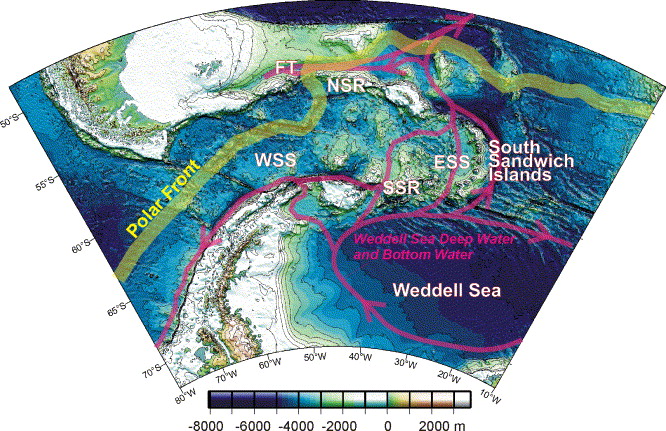
Drake Passage
Cape of Good Hope

More nose holding: Winds Seen As Key Driver Of Antarctica’s Growing Sea Ice
Disentangling the actual data from the CAGW hype is a royal pain in the neck sometimes.
And saving the best for last:
Salvatore Del Prete says: June 21, 2014 at 3:38 pm
Every time I would post a study supporting solar/climate connections Leif would say it was out dated and no longer valid . Even if they were as recent as a year or two ago.
>>>>>>>>>>>>>
Yes that is why I finally gave up.
I also noticed when he took a potshot at me and I told him to go fight it out with Dr. Nir Shaviv
…CRICKETS…
Someone mentioned LS criticism to Dr. Nir Shaviv and he rebutted BTW.
See comments @
http://www.sciencebits.com/calorimeter
Hi TB:
I went through all the Niños and Niñas since 1870, identified when they occurred relative to the phase of the solar cycle and plotted the results on a histogram (I’ve plotted two solar cycles to make it easier to see what’s going on):
The results show most Niños and Ninas beginning quite abruptly just after solar maximum, continuing through solar minimum and dying out about half way up the leading edge of the next solar cycle. According to binomial stats the chances that this pattern is a random event are on the order of 10:1 against.
To me this is good evidence for an ENSO/solar connection. I’ll leave you to figure out the details. 😉
Hi Roger A: Thanks for this. We do have to account for the rise time being shorter than the decline time on the solar cycle though. The sine wave needs skewing a bit, unless you’ve treated the data is some clever way I haven’t spotted? Landscheidt reckoned the split was on the golden section. So in a random distribution, there would be a 1.618 times greater chance of an event being on the declining side of the cycle.
Carla says:


June 20, 2014 at 7:45 pm
Helio current sheet is also, also, taking longer to complete its contribution to the solar cycle. nooo
Please note for the year 2001.
Such was, by comparison, the temperature of the ozone zone in 2000.
In contrast, as in 2002 and similarly in subsequent years.

TB:
I calculated phase angles by setting solar minimum to 0 (360) degrees and solar maximum to 180 degrees for each individual solar cycle, so the plot allows for solar cycle asymmetry.
I don’t think Landscheidt’s 1.618 ratio applies here because the “split” between frequent/infrequent Niños & Niñas doesn’t occur at solar maximum and minimum.
Roger A: Hmmm, need to think about that a bit. Maybe you’re right, but visually is does misrepresent a bit. As I said to Salvatore, the important thing is to see which pahse of the solar cycle the ENSO events are initialised in rather than the phase when they are at their peak.
Ren: You are comparing a deep La Nina year (2000) with sustained El Nino years
TB: I already did that. 🙂 Here are the results. I’ve plotted the earlier “peak amplitude” graph at the top for comparison purposes:
You can see a sharp drop in temperature over the equator in 2001, in the lower stratosphere.


Such was the temperature from 1997 to 1998.
At the turn of 2013 and 2014 the temperature has increased significantly, but again decreases. There were chances for El Niño, but the situation is changing.
You can see a clear effect of solar activity on the temperature of the equator. At the turn of 2013 and 2014 activity was high. Activity fell and the temperature dropped.

Roger Andrews, thanks for sharing those graphs. They remind me that way back whenever I looked into this quickly (years ago) I knew a lot less about climate (especially circulatory topology) & multiparameter wavelet customization than I know now, so maybe I’ll revisit this sometime. The first thing I’ll be checking (which almost no one in the climate discussion ever bothers to check, thus quickly undercutting the trust I’m naturally inclined to extend in good will) is whether the implicit temporally-global binning assumption holds. Again: Thanks for sharing stimulating summaries.
Also an update for everyone: I’m delaying the release of my latest solar-terrestrial-climate explorations. I found another variable that dovetails in, so it takes time to include it. For those of you who don’t yet know, I’m working on SAM. SAM is the ruthless murderer of AGW.
FROM LAYMAN SUNSPOT SITE the article below.
This is what I have been saying which is the sun has more solar variability then what mainstream leads you to believe in.
opening Figure on this article shows a graph from Lockwood showing solar output over the last 400 years. The blue line is his new suggested solar output that takes into consideration the “Waldemeir Discontinuity” along with the “Wolfer Discontinuity” and the “Wolf Discontinuity”, he also suggests the red line (based on the GSN) is just as likely to be correct. The Lean (2000) TSI reconstruction is very close to the Lockwood solar reconstruction (Rc) and the GSN record (Rg) which will have huge ramifications if correct, it will reveal that the Sun has had a bigger variance in TSI over the sunspot record that is far greater than the 0.1% that Svalgaard and the IPCC subscribe to.
Roger A: Excellent! The iinitialisation graph pretty much vindicates my long held position (take note Paul 😉 ) on ENSO magnitudes being in antiphase to the solar cycle, and so flattening the solar signal in the temperature record. It also shows why 2014 was never going to be a big el Nino year; we’re at solar max, even if it’s a small cycle.
Paul Vaughan says: @ June 21, 2014 at 9:22 pm
“… For those of you who don’t yet know, I’m working on SAM. SAM is the ruthless murderer of AGW.”
>>>>>>>>>>>>>>>
I take it that SAM = the Southern Annular Mode.
As in the paper I just referenced: Eddy response to Southern Ocean climate modes
I am not at all surprised that SAM murders AGW.
Gail, I doubt it. If you think you know what one of Paul’s acronym’s stands for, you don’t. 😉
I’ll go for Solar Asymmetric Modulation
Thanks T.B. That is the trouble with abbreviations. (I bet they are connected via changes in ozone.)
‘Also of interest is that the period is 1/8 of the lunar ‘Saros’ eclipse cycle of ~19yrs.’
19 years is the Metonic cycle. Saros is 18.02933 years.
Thank OB: I’m always mixing those two names up
TB: Pleased to hear that you and PV liked the last graphs. You should find the next one even more interesting.
I decided I didn’t like the “event initiation” plot because I’d picked “initiation” at the point where the Niño3.4 index crosses the +/-0.5 thresholds commonly used to define Niños and Niñas. As well as being arbitrary these thresholds also ignore the fact that in many cases the Niños and Niños had been building for months before they crossed them (the 1997 Niño started to build four months before it crossed the +0.5 threshold and the 1998 Niña effectively started to build up (down?) as soon as Niño3.4 turned over after the peak of the 1997 Niño, six months before crossing the -0.5 threshold).
So I went back and picked “lift off” points where breaks in Niño3.4 define when the Niños and Niñas really began, plotted them against solar cycle phase, and here’s what I got:
Looking better all the time 🙂
Thanks for the update Roger Andrews. I was already convinced to look — now even more so.
–
I managed to finish the Sun & SAM article, crushing my previous records for being concise (1 pulverizing page).
I’ve sent it off to Bill Howell, who has been generously hosting some of my work since I left SFU (and the perks I used to take for granted there, like access to 1/2 million dollar annual software site site licenses, computing accounts, etc.)
I think that since the temp ramp rate is higher entering the interglacial than when entering the glacial, this would cause a slow temp increase when the climate is driven with a 50% duty cycle. Its ALL about the time constants, from enso to amo…maybe even the 1200 yr cycle. Great discussion…still can’t believe its labeled settled science without an understanding of the ocean response, considering our planet is 70+% water..
@Roger Andrews: impressive, hats off 😎 does your ‘decalibration’ also mean you dropped the Running 3-Month Mean ONI values and plotted just the data?
http://ggweather.com/enso/oni.htm
Such a circulation in the lower stratosphere over the equator cools. What’s more will fall possibility of formation of hurricanes.
http://earth.nullschool.net/#current/wind/isobaric/70hPa/orthographic=-108.32,4.76,635
Roger A: Thanks for the further analysis. I think as well as your study of numbers of ENSO events it would be worth doing a separate analysis for their amplitudes in terms of released/absorbed energy too. But this is tricky, given the underlying PDO. I believe that will reveal that the energy relationship between solar energy in and ENSO energy out is nearer to antiphase than your event numbers graph reveals, because the ENSO swings get bigger as the cycle declines to minimum, and because the big El Nino occurs near solar minimum, the following La nina occurs near solar maximum. I’ll have a think about designing the analysis. Firts thought is to exclude or somehow filter big volcanic eruptions which confound the analysis by precipitating El nino.
Roger A’s plot of ENSO event frequency against solar cycle phase at the time of the event’s origin:

For sure the volcanoes are coupled in, as I’ve shown before:

But for the same reason I lost interest in the IPO forecasting that I determined was feasible, I’ve already lost interest in pursuing this solar-ENSO stuff overnight: ENSO (including interdecadal IPO which is yet another order of magnitude smaller) — regardless of whether mostly solar or mostly lunisolar — only accounts for 18% of the variance and I’ve already proven geometrically that it isn’t necessary to solve the ENSO puzzle to know for sure what’s going on with the other 82%.
I operate on the Pareto Principle (80/20 rule for using time & resources efficiently). I’ve already overshot my target at 82/18.
So I’m leaving it on the backburner. I’m not sure what can cause me to make it a priority — perhaps only secure longterm pay & pension at the local university.
But I’ll watch with interest as others attempt a far more inefficient equivalent to the aggregate proof I’ve already given. (There’s a lot I could say about David Evans’ interpretation of notch & lag. I’m just not saying it.)
We each have a different role to play. Sincere thanks to everyone for contributing. The Talkshop is for sure the best place currently available to discuss the sun & climate.
Thanks to Roger Andrews for providing the highlight of this thread. I look forward to watching Roger Andrews’ explorations evolve.
Paul V: In the current political context the demands of formality suck inordinate amounts of time & energy and the payback is biased rejection, harassment, & hatred, so it’s a fool’s errand IMO.
The result of the harassment we got for our PRP special issue from the IPCC authors and team WUWT resulted in our papers being downloaded thousands of times more than they would have been otherwise. Monthly counts are still high. 🙂
Chaeremon, you ask: “does your ‘decalibration’ also mean you dropped the Running 3-Month Mean ONI values and plotted just the data?”
I used Kaplan and Reynolds Niño3.4, not ONI (although all the Niño indices are very similar) and I applied the five months duration, +/- 0.5 threshold, 3-month smoothed criteria in all cases to keep the playing field level. (Note, incidentally, that applying these criteria makes a number of the smaller Niños TB identified in his “plot showing positive ENSO events in relation to the solar cycle” go away and increases the Niño “quasi periodicity” from 3.7 to 4.1 years.)
TB: Our definitions of what’s desirable certainly differ on that one. I assure you that I respect your perspective. I’m curious: Do you get paid royalties? (If I was and they were substantial, I’m practical enough that I’d look at this differently.)
Hi Paul: No, not a penny. I’m doing what I do to defend science. That is all.
Here, too, the historical data. It may be differently.
http://www.cpc.ncep.noaa.gov/products/analysis_monitoring/ensostuff/ensoyears.shtml
_
Another solar-terrestrial-climate mystery solved:
Sun & SAM
Sunspot Integral & Southern Annular Mode (SAM)
Gail wins the PV acronym competition! 🙂
Thanks Paul.
If happy to share, what did you find the ‘SST neutral’ sunspot number to be for the SAM?
In my original study, I found it was around 40 for the globally homogenized SST.
TB:
SAM Reconstruction: ~50 (r^2 = 90%)
ERSSTv3b2 90°S-8°S: ~46 (r^2 = 86%)
ERSSTv3b2 90°S-8°N(thermal equator): ~45 (r^2 = 83%)
You see the problem here:
ERSSTv3b2 90°S-90°N: ~43 (r^2 = 77%)
ERSSTv3b2 8°N(thermal equator)-90°N: ~37 (r^2 = 52%)
As I have proven geometrically:
There’s no proper accounting for the northern hemisphere without SCD = solar cycle deceleration.
Via Milankovitch, Sidorenkov’s section 8.7 can be extended to include the solar cycle and correct the error in this paper:
Thomson, D.J. (1995). The seasons, global temperature, and precession. Science 268, 59-68. doi:10.1126/science.268.5207.59.
Click to access 228341-2886492.pdf
Jean Dickey is the only American I would trust to supervise such work, but she works for the US government, so unfortunately I suspect that her flexibility & freedom is fatally compromised.
With regard to ocean heat content and solar variance, this 2004 paper has some relevance –
“Impacts of Shortwave Penetration Depth on Large-Scale Ocean Circulation and Heat Transport”
http://journals.ametsoc.org/doi/pdf/10.1175/JPO2740.1
While the paper is modelling based and is largely concerned with biological turbidity, the physical mechanisms proposed would have similar effects to solar variance in strength of UV penetrating to depth.
It is notable that the authors understood the difference between “near blackbody” and “selective surface” and thereby why the depth of absorption was critical to heat content and circulation patterns.
The basics of such “selective surface” effects on temperature can be demonstrated with very simple empirical experiments –
PV – re Sun & SAM – “it’s a beautiful thing”.
The admirable thing about the Talkshop is that people here actually figure things out. You’d think after all these years, the others would have made some actual headway….
Today 10.7 flux is 101, just about the threshold in question, plus or minus a few photons, and US temps are following suit here just past the solstice (until solar farside active regions roll back into view and flux goes up again short-term a bit followed by temps).
The true nature of reality will be glaringly obvious as SC24 really starts to wind down.
The world will soon be freed from the death grip of the willfully ignorant, thanks in part to Tallbloke’s Talkshop.
Thanks TC. Glad l am not the only one who I feeling a bit uneasy about the conclusions
.
Nice work RogerA.
The’ lift off point’ graph is the neatest and most interesting for sure.!!
It appears Defining ENSO from ‘lift off point’ sounds good practice for cycle analysis.
opens up a whole new field of ENSO research really
Cycle research uses the peaks/troughs ..but we measure ENSO by human determined thresholds. ( +/- 5 ..a cross section of the cycle. No wonder your graph shows symmetry. It is drawn to pursue cyclical behaviour rather than percentiles
curiously…

The solar cycle histogram shape is the same shape as the ENSO frequency distribution and that bedazzled me.
It looks like the ENSO histogram ‘copies’ the solar cycle ‘histogram’ with a 90 deg lag.
It sort of looks intuitively like an echo l thought…
Just another way at looking at your graph.
Bob, thanks for your kind words. It make the (unpaid) effort that much more worthwhile.
Konrad: Thanks for that paper. I didn’t realise so much of the downwelling shortwave energy (40%!) absorbed in the ocean was in the shorter wavelengths. I was taken in by Svalgaard again.
Have you ever seen a graph of global temp’ with a 13 yr trend
graph by bob Tisdale
https://picasaweb.google.com/110600540172511797362/TIMESERIESAndTrends#6026214543743014114
There’s those saw tooth wave ‘cliff edges’ again . Step like changes./inflection points
How does this 13 yr trend data line up with solar cycles? 13 yr trend is closer to the 11 yr solar cycle .
Am l reading right Roger A.
From your graph. ENSO never occurs at 70-100 deg ?
What does this mean ?
WC: Not sure what Bob has done with the data there. Have you a link to the OP?
Paul: Thanks for the breakdown. I agree that another factor needs to be included for the Northern Hemisphere. I wonder if the AMO and North Pacific cycles might help account for the swings.These oscillations are in phase with heliomagnetic changes anyway.
WC: The data Roger A has used shows ENSO events don’t occur once the upswing of the solar cycle is under way, until it’s at around max. I’m not sure why, for e.g., the big La Nina following the 97/98 El Nino doesn’t count.
TB: SCD = geometrically proven
tallbloke says: @ June 23, 2014 at 1:19 pm
….I didn’t realise so much of the downwelling shortwave energy (40%!) absorbed in the ocean was in the shorter wavelengths. I was taken in by Svalgaard again.
>>>>>>>>>>>>>
Over at WUWT I kept posting these graphs which I think shoot dead L.S. constant sun, nothing to see here move along crap:
(Colorado Laboratory for Atmospheric and Space Physics killed my original link to that graph BTW, and sent you to one of their CAGW be VERY AFRAID sites instead.)
This graph is the real killer:

Paul: Sure, but we eventually need to trace the line from ultimate cause to proximate cause. Magnetism, ocean currents, ozone, clouds, etc.
Gail, adding, there is a UV window through the atmosphere.
The sun like so many other things is looked at simplistically. The mean of radiation varies little but there is a spectral shift.
There is more.
In addition there is interaction with the high atmosphere too and indirect effect (spectrally shifted there)
TB: insolation gradients = proven (via laws of large numbers & conservation of angular momentum)
I realize people haven’t digested this. I am at peace with this.
Check out the graphs in my last post and then add in NASA’s info. and file under the sun is constant and the science is settled label. {:>D
In this article Mankind of course is to blame for the increased UV and not the sun. Typical CAGW fantasyland.
That interpretation is contradicted by these articles from NASA
Yet despite this information, five years later they find their estimates are off by “a factor of four to six larger than expected”
tchannon you were saying: “… The mean of radiation varies little but there is a spectral shift.” While I was scrounging up the NASA articles supporting your statement.
To me L.S. denial of the sun’s affect on current short term climate is completely mind boggling in the face of all the evidence to the contrary.
Paul: Insolation *at the surface* varies with cloud more than with solar variation. I strongly suspect there’s a link, and that it is the amplification mechanism needed to get from TSI (or it’s components) to observed change, but I think ‘proven’ is a claim too far at the moment. If you feel your work has proved it, then fair enough. The rest of us will plod along with our study until such time as someone pays you enough to explain it to us so we can agree or ctiticise.
tallbloke, If you read those NASA articles, you will see the UV cycle is a half cycle off from the Sunspot cycle just like the ENSO cycle is a half cycle off from the Sunspot cycle…. HMMMmmm
That can be followed back to the fact that most of the world’s oceans are in the southern hemisphere and that ozone affects the Antarctic polar winds per one of my other recent comments.
If you look at this Sea Surface Temperature map it has a good image of the tongue of cold water from the Antarctic Circumpolar Current just before Drake Passage, headed up the coast of South America to Galapagos.
fhhaynie (former EPA scientist) says: @ January 18, 2014 at 8:24 am
The same happens along the coast of Africa and effects the gulf stream.
Another interesting WUWT comment
I think all the emphasis on the Arctic is massive misdirection.
TB: I must reiterate to ensure clear reception:
insolation gradients (not simply insolation)
(It’s the gradients that drive flow & mixing.)
The proof applies to a unit.
You express interest in subdivisions of the unit.
That’s all I have time for today. (The paid-work week is underway.)
Paul: I too am interested in how rates of change (gradients) of insolation affect weather and climate. See for example the latest post on El Nino and Luni-solar connections. – When The solar cycle starts to fall steeply – El Nino is precipitated. When the solar cycle stops falling, El Nino is precipitated again.
My approach is more qualitative than your statistical appraoch, but I think both approaches are needed to unearth the hidden climate connections.
TB:
Re your comment of June 22, 2014 at 1:06 pm
Defining the amplitudes of Niños and Niñas is tricky not because of the PDO but because of two problems with the Niño indices themselves – 1) the use of arbitrary thresholds and 2) the fact that the indices are suspect before ~1950 because of the way the SSTs used to define them have been spindled, folded and mutilated by “corrections” before then (which is why Multivariate ENSO goes back only to 1950). We can get around problem 1) by calculating “released energy” during an ENSO cycle without using a threshold, as you suggest, but problem 2) is less tractable. One possible solution might be to use the SOI index, which having suffered fewer “corrections” should be more robust than the Niño indices before 1950 and which marches pretty much in lockstep with ENSO. (Which comes first? I say ENSO, by about a week) 😉
Another important point to remember is that Niñas contribute just as much to the heat release process as Niños. Bob Tisdale has discussed this in a number of posts:
And I added my ten cents’ worth in a post a couple of years ago. First how the upswing in temperatures is delayed until the end of the Niña:
Second, how the Chichón eruption failed to stop the 1983 Niño, which lifted off several months before the eruption, plus another delay in the temperature increase until the end of the last Niña in the sequence:
And third, how the Pinatubo eruption made only a minor dent in the 1991 Niño, which also lifted off before the eruption, plus how the 2002 Niño, which didn’t transition into a Niña, had no visible impact on temperature.
The conclusions I draw from these and other plots are:
* We get heat release only when a Niño transitions into a Niña – Niños by themselves don’t release heat.
* So we can’t concentrate solely on Niños. Niñas are just as important.
* ENSO events don’t much care about volcanic eruptions, so there’s no need to “filter them out”.
Gail, TB, PV etal – it is so much much fun watching here. There are a few more cards to be played and it’s game over. If I wasn’t constructing my electricweatherdotcom website right now, I’d happily pass you those cards (I’d like to save *something* new for it!). – hopefully before you find and play those cards yourselves! …LOL – what a joy it is knowing you’re (all) here. This is not really a competition, ’cause we’re all in this together!
Svalgaard etal – jeez – how does that happen? By design? By accident? Density? Who knows – who cares. Soon he and AW should completely understand the true nature of solar influence. It’s not as though they haven’t had every opportunity. Unless they choose to DENY objective reality….
Climate Factors Colder Overall When Viewed Objectively
Milankovitch Cycles- favorable for glaciation presently and for the next 4000 years.
Solar Activity – favorable for colder temperatures post 2005 and continuing until at least 2030.
Solar activity will be high favorable for cooling once the weak maximum of solar
cycle 24 ends, Will be in the very near future.
Ocean/Land Arrangements- highly favorable for glaciation and colder temperatures presently
and well into the future.
Solar Secondary Effects- neutral for cooling during the weak maximum of solar cycle 24 will
become highly favorable going forward when solar cycle 24 maximum
ends.
Lunar – neutral. I don’t see a strong connection with this factor hence neutral.
Commentary welcomed.
CO2 – unknown. Higher then when past glaciations were initiated through
Milankovitch Cycles but unknown if glaciation would have occurred
back then if CO2 concentrations would have been higher.
Ice Dynamic – unfavorable ,since most of the large ice sheets form the last N.H.
ice age are gone. Still Greenland is a source.
Earth Magnetic Field- neutral but will be heading toward favorable as this keeps weakening
gong forward into the future.
When one looks at this picture presented in the above I think it is safe to say the climate is not heading for warmer times but rather toward colder times and the possibility of a return to glacial conditions sometime in the not very distant future is possible.(0- next 4000 years )
‘the sun’s output actually fluctuates in sync with changes in the sun’s magnetic field’
Remember that one, it won’t be promoted by ‘official climate science’ any time soon.
Roger A: Thanks for the extensive comment. First, let’s clear up a misconception about volcanos. I think they need not so much filtering, which implies an automated process, but scrutinizing. If anything, I’d expect them to augment, not diminish and El Nino. here’s why:
My hypothesis rests on the idea that El Nino is precipitated by a drop in solar activity (probably accompanied by an increase in cloud). When the Sun turns down the heat from above, the ocean starts releasing the excess energy it absorbed during the high part of the solar cycle. This results in an increasing amplitude train of ENSO events as the energy burps out, ending with the big El Nino at solar minimum and its consequent following La Nina heading towards solar max.
So if – and it’s an if – a volcano causes a significant dust veil, reducing insolation, it should also help precipitate or augment an El nino event.
Since both big volcanos of the satellite age went pop just as the solar cycle started to fall steeply, we won’t be able to quantify effects for some time to come. I just hope Katla doesn’t blow in the next few years. Good for science, bad for crops.
Bob: Being an ol’ time engineer I try to explain as much as I can with simple thermodynamics. Doubtless there are some important electrical effects at the solar energy terrestrial interface that quickly gets into upper atmospheric chemistry I don’t pretend to know much about. I look forward to your website going up so we can see what you’ve got.
http://iceagenow.info/2014/06/confirmed-earths-protective-magnetic-shield-weakening/
Rog, if I remember correctly it depends at what latitude the volcanic eruption occurs.
Low latitude volcanic eruptions promoting El Nino. I don’t know about high latitude volcanic eruptions in this regard.
However many studies have shown that major geological activity equates to prolonged solar minimum activity .
In addition high latitude volcanic eruptions will promote a more meridional atmospheric circulation because they warm the stratosphere more in the higher latitudes relative to lower latitudes.
Salvatore: Yes, that’s why Katla is a danger to North Hemisphere. Meridional loopiness in the jetstream means extreme cold events. Frost kills crops.
Right. I have to attend a UKIP committee meeting. Back later after we’ve planned the revolution. 🙂
This is the only site that is tackling why and how the climate changes in a comprehensive very scientific objective way.
The questions as to why the climate does what it does are only really being addressed here with no agendas to be found just scientific paper after paper.
TB: lt all starts with the Sun’s electric and magnetic fields. From there it’s fluxes of photons, protons, and electrons. At the Earth it’s the magnetosphere, the ionosphere, and the global electric circuit. Straight heat transfer, thermodynamics, and circulation covers the response to variable photon heating. There’s mountains of evidence to support your works and mine, including sensible testable mechanisms that you and the “crew” have diligently discussed for years. Lotsa credit to go around.
Let’s face it, there is only one reality, objective reality, and we just want to know what it is, don’t we?
TB: See if you can match Niños up with eruptions 🙂
Rog, this came out today on WUWT. Maybe this could be run on your site so we can trash it. What utter nonsense. Then again maybe it is not worth the time of day.
.
Maunder and Dalton Sunspot Minima
Posted on June 23, 2014 by Willis Eschenbach
Guest Post by Willis Eschenbach
Bob W: there is only one reality, objective reality, and we just want to know what it is, don’t we?
Yep.
Salvatore: This is the only site that is tackling why and how the climate changes in a comprehensive very scientific objective way.
We try not to get distracted on these analysis posts. Due to blog policy, the competent pro co2 theory people tend to keep a low profile when they know they are not going to be able to disrupt discussion of natural forcings. Those that get to comment here that is. The trolls have been shown the door.
Maybe this could be run on your site so we can trash it. Then again maybe it is not worth the time of day.
Willis is one of the trolls who got shown the door. Thankfully he launched himself through it without me having to apply the boot. We do occasionally rip one of his posts apart, but that one is such a pile of trash I won’t waste time with it .
I think that is the correct policy. Why acknowledge something as absurd as what he says in that article..
Gail Combs says:
June 23, 2014 at 2:51 pm
————————————
Gail,
very interesting finds.
UV variance casing ozone changes thereby effecting surface UV could be amplifying surface UV variance further than simple solar spectral variance may indicate.
Surface UV changes of 10% is huge given that UV-A still has the power of 10 w/m2 at 50 m depth in some waters.
While it is possible to empirically demonstrate the changes in heat content of a water column due to such changes, because of the +100m depth required, this would be expensive.
However there maybe sufficient real world data available from the ARGO buoys. Their deployment covers the end of SC23 and the start of SC24. It may be possible to identify the solar signature in data from below 100m. (SSTs are too noisy for short term signals). The question would be just how badly Josh “cold enough for ya” Willis and Co. have corrupted the ARGO data….
Salvatore Del Prete says:
June 23, 2014 at 8:42 pm
———————————-
“Then again maybe it is not worth the time of day.”
I’d leave it at WUWT where it belongs.
The storm of “red thumbs” at Jo Nova seem to have sent the JCB into a digging frenzy. Next post could be a postcard from China. Something good may come of it. He might unearth Maurice Strong 😉
Of course there could be method to the madness. He started that hole back in 2011. If it gets deep enough he may no longer have to see the annoying light of our variable sun…
Konrad, the important Argo data will not be the obvious. Of far greater importance is discovering the circulation patterns (includes z-axis) and layering. This is an extremely fierce 4D+ problem.
I do have a suggestion to do with the sea patterns, a subject I rarely consider. Where to put this and how to try and describe it is open, not decided.
tchannon says:
June 24, 2014 at 12:32 am
———————————–
“This is an extremely fierce 4D+ problem”
Agreed. The Z-axis issue would likely confound identification of a global signature for such a short time series as ARGO. However a regional signature demonstrating the mechanism may still be identifiable.
What would be needed –
Uncorrupted ARGO data with outliers re-included.
A region with little upwelling or downwelling in the 100 to 700m layer.
A region with little variance in biological or mineral turbidity.
A region removed from the cloud confusion of the ITCZ.
Given that ARGO is global this would be difficult but not impossible. I suspect what would be necessary is to “track” a water mass across the selected region. ARGO floats spend more time at depth than at the surface, however while at the surface they are subject to faster wind driven surface currents. To track a water mass below 100m, gridded data would be needed, with below 100m temp data selected to match below 100m flow as determined by resurfacing positions of individual floats.
TB: I need to concisely clarify further:
spatial gradients (not temporal derivatives)
specifically equator-pole & consequent mid-latitude westerlies, particularly in the winter hemisphere (e.g. Dickey, Sidorenkov — accessible via link trail I give from Sun & SAM article above for anyone ready for dead serious study of the proof)
apologies — during the paid-work week I necessarily drift out of the conversation, so I suggest we leave it there since my availability is too low to avoid serious misunderstandings
Again: Thanks for hosting the best solar-terrestrial blog. I look forward to more in depth discussion as/when time permits.
–
Bob: Thanks for your comments.
Gail: I quoted you at JoNova’s (about controlled opposition).
Salvatore Del Prete says: @ June 23, 2014 at 5:25 pm
“…Lunar – neutral. I don’t see a strong connection with this factor hence neutral.
Commentary welcomed…”
This is a subject I have only a glancing knowledge of but I do not think it should be dismissed.
LUNAR
There is some indication that the north/south vector of the moons position related to the earth could be the cause of D-O/Bond events:
On the 1470-year pacing of Dansgaard-Oeschger warm events This warmist paper says the lunar cycle is 1800 years and therefore can not be the culprit. However The 1,800-year oceanic tidal cycle: A possible cause of rapid climate change by Charles D. Keeling and Timothy P. Whorf say lunar tides are a possible cause.
“…. It takes between 1226 and 1550 years for the members of a saros series to traverse the Earth’s surface from north to south (or vice-versa)….” ~ (wwwDOT)absoluteastronomy.com/topics/Saros_cycle
A blog essay on the subject: Are the Dansgaard-Oeschger (D-O) Warm Events driven by Lunar Tides? astroclimateconnection.blogspot(DOT)com.au/2013/06/are-dansgaard-oeschger-d-o-warm-events.html
and another by E.M. Smith: The Moon’s Orbit is Wrong, It Can Change a Lot, And Tides Will Too (with links to several of his other lunar essays -all worth reading)
chiefio.wordpress(DOT)com/2014/01/24/the-moons-orbit-is-wrong-it-can-change-a-lot-and-tides-will-too/
Also on that 18.6 year cycle:
The influence of the lunar nodal cycle on Arctic climate
ABSTRACT
…The paper presents an analysis of the time-series for the polar position, the extent of Arctic ice, sea level at Hammerfest, Kola section sea temperature, Røst winter air temperature, and the NAO winter index as a way to identify a source of dominant cycles. The investigation uses wavelet transformation to identify the period and the phase in these Arctic time-series. System dynamics are identified by studying the phase relationship between the dominant cycles in all time-series. A harmonic spectrum from the 18.6-year lunar nodal cycle in the Arctic time-series has been identified. The cycles in this harmonic spectrum have a stationary period, but not stationary amplitude and phase. A sub-harmonic cycle of about 74 years may introduce a phase reversal of the 18.6-year cycle. The signal-to-noise ratio between the lunar nodal spectrum and other sources changes from 1.6 to 3.2. A lunar nodal cycle in all time-series indicates that there is a forced Arctic oscillating system controlled by the pull of gravity from the moon, a system that influences long-term fluctuations in the extent of Arctic ice. …
E. M . Smith last essay on the moon/s affects on the climate A Remarkable Lunar Paper and Numbers on Major Standstill
chiefio(DOT)wordpress.com/2014/01/25/a-remarkable-lunar-paper-and-numbers-on-major-standstill/
Salvatore Del Prete says: @ June 23, 2014 at 5:25 pm
“….CO2 – unknown. Higher then when past glaciations were initiated through
Milankovitch Cycles but unknown if glaciation would have occurred
back then if CO2 concentrations would have been higher….”
The CO2 record is more mucked-up, b@$tardized and generally mangled than the temperature record and that is saying a lot!
For example CO2 measured up to 640 ppm in 1939/1940
(wwwDOT)biokurs.de/treibhaus/literatur/kreutz/kreutzwspapprox.gif
Probably the worst problem is the ASSumption that CO2 is well mixed. It is not.
In the paper by Tom Quirk “ Sources and Sinks of Carbon Dioxide” The isotopic balance in the atmosphere is far more complex and there are many more variables than most think. Consider 94% of all anthropogenic CO2 is released into the northern hemisphere. Next the CO2 is not as well mixed as the IPCC state. From the nuclear tests in the 60’s the mixing north to south is very slow, like several years ( another rhetorical question) so why is the average northern hemisphere CO2 not higher than the south?
As Dr. J. A. Glassman so aptly put it in one of his replies,
The AIRS satellite shows it is not well mixed and the CO2 is similar in the Norther and Southern Hemispheres:

The key is that “AIRS reports the daytime and nighttime global distribution of carbon dioxide in the mid-troposphere at a nadir resolution of 90 km x 90 km” and they STILL do not have uniform CO2. The Japanese Satellite (JAXA) Data shows even more variation.
Some links on the subject:
CO2: The Greatest Scientific Scandal of Our Time by Dr. Zbigniew Jaworowski
http://www.warwickhughes.com/icecore/
(click on the various pdfs)
Dr. Glassman’s rebuttal of the ‘science’ of CCo2
http://www.rocketscientistsjournal.com/2006/10/co2_acquittal.html
(wwwDOT)rocketscientistsjournal.com/2007/06/on_why_co2_is_known_not_to_hav.html#more
This comment at Steven Goddard’s Includes my experience with IR spectrophotometer in the 1970s, the instrument used by Keeling- There is no way you can get an accuracy of parts per million with that instrument!
http://stevengoddard.wordpress.com/2014/03/25/coldest-october-march-in-the-us-in-102-years/comment-page-2/#comment-333230
Salvatore Del Prete says: @ June 23, 2014 at 5:25 pm
“….Ice Dynamic – unfavorable ,since most of the large ice sheets form the last N.H.
ice age are gone. Still Greenland is a source….”
It is not the amount of ice but the rate of growth in the ice/ snow cover that matters. As RACookPE1978 said on December 31, 2013 @ WUWT:
Long term glaciers that had melted away during the Holocene Optimum have reestablished.
Temperature and precipitation history of the Arctic 2010
A new approach for reconstructing glacier variability based on lake sediments recording input from more than one glacier January 2012
Perhaps more important is the dynamics of energy loss. Again RACookPE1978 does a great job of explaining that.
A more detailed comment @ wattsupwiththat(DOT)com/2014/02/18/how-much-sunlight-actually-enters-the-system/#comment-1571201
and Cook’s table on “Direct Radiation Horizontal Surface”.
The radiation received on the equinox for solar radiation at each latitude at noon.
http://wattsupwiththat(DOT)com/2014/02/17/crises-in-climatology/#comment-1571641
And do not forget The Earthshine Project at Bigbear Observatory showing a change in albedo – graph
Salvatore Del Prete says: @ June 23, 2014 at 5:25 pm
“….Earth Magnetic Field- neutral but will be heading toward favorable as this keeps weakening
gong forward into the future…..”
Ice Age Now site has:
Confirmed – Earth’s protective magnetic shield is weakening:
There is also quite a bit of snowy weather reported not only in South Africa, South America, New Zealand, Australia but also in Turkey, Russia, Estonia, Finland, Norway, Sweden, and the Rockies. Also reported is record cold in Oregon, Romania, Seattle and Finland and “Snow is still persisting in the low north eastern Italian Alps”
Not to mention five Aleutian volcanoes now simultaneously active – the most activity in 26 years.
Amazing how we only see reports of the Warmest Spring Evah…
It is so nice that Ice Age Now collects all the information we would never see otherwise.
tallbloke says: @ June 23, 2014 at 5:31 pm
“…..My hypothesis rests on the idea that El Nino is precipitated by a drop in solar activity (probably accompanied by an increase in cloud). When the Sun turns down the heat from above, the ocean starts releasing the excess energy it absorbed during the high part of the solar cycle….”
Remember Tallbloke, NASA found
And a companion paper: Climate sensitivity to the lower stratospheric ozone variations
SAM and ozone: Decadal Changes of Wind Stress over the Southern Ocean Associated with Antarctic Ozone Depletion.
So throughout the solar cycle there is a shift in the wavelengths from deep ocean penetrating UV to shallow penetrating visible, near infrared. This would shift the part of the ocean that is receiving energy and heating up. On top of that is a change in the wind that drives the Antarctic Circumpolar Current because of changes in ozone.
I would think that the changes in those two factors, ozone and the ocean depth the solar energy is heating, could drive ENSO. (I haven’t put in a lot of time disentangling the info on these two factors.)
Drat, sorry Tallbloke, I am half asleep and messed-up the blockquotes.
[mod: I’ve added a couple of unquotes but quite what is wrong is err… maybe it will do –Tim]
Bob Weber
“TB: lt all starts with the Sun’s electric and magnetic fields. From there it’s fluxes of photons, protons, and electrons. At the Earth it’s the magnetosphere, the ionosphere, and the global electric circuit.”
Hear, hear 🙂
I look forward to seeing what you have got – though I would consider it as light atoms (photons), positively charged atoms (protons) and negatively charged atoms (electrons) 😉
TB said
WC: The data Roger A has used shows ENSO events don’t occur once the upswing of the solar cycle is under way, until it’s at around max. I’m not sure why?
[Mod note] This isn’t what I said. What I said was: “WC: The data Roger A has used shows ENSO events don’t occur once the upswing of the solar cycle is under way, until it’s at around max. I’m not sure why, for e.g., the big La Nina following the 97/98 El Nino doesn’t count.”
—-
The first thing that comes to mind is the period in time when the atmosphere is not in phase with the ocean and does not ‘couple’ Just like our current ENSO state now . We have had neutral years as the up phase of solar is in progress.
We could predict that we will have La Nina or El Nino after solar maximum according to Andrews frequency distribution histagram
But this cycle 24 is unique. It is likely to have a double max solar peak as is the case at the start of every 3rd schwabe triplet when the ~66yr cycle reaches max and min
Also a long solar cycle predicted l believe. So maybe some more neutral years to come before we hit the downslope of solar cycle.
Link to OP? what is that? ( I always place links on pictures not my own) read the bottom of pic’
[Mode note] OP= Original post. In this case, the post by Bob Tisdale.
From the bottom of that picture of the13 yr trend of global temps’ l posted from B Tisdale
link to OP
WC: Thanks.
“An explanation of what’s being presented in Figure 6: The last data point in the graph is the linear trend (in deg C per decade) from January 2001 to May 2014. It is basically zero (about 0.02 deg C/Decade). That, of course, indicates global surface temperatures have not warmed to any great extent during the most recent 160-month period. Working back in time, the data point immediately before the last one represents the linear trend for the 161-month period of December 2000 to April 2014, and the data point before it shows the trend in deg C per decade for November 2000 to March 2014, and so on.”
Gail, thanks for al the great info. again.
Salvatore, no problem. I hope you can use it to beef-up you theory.
Gail part of a paper you sent. It shows much doubt about the 1470 year climate cycle and has no concrete reason for it ,if it does exist. Interesting however…
[18] If the 1470-year pacing cycle would originate from astronomical fording, the long-term stability of the orbital elements within the solar system make them a prime candidate for generating the 1470-year pacing cycle. So far, a periodicity of ∼1800 years has been identified [De Rop, 1971; Keeling and Whorf, 2000], which arises from the periodic motions of Earth and Moon and may modulate large-scale oceanic mixing by variations in the strength of oceanic tides. Keeling and Whorf [2000] proposed a mechanism by which these tidal variations induce changes in climate and suggest that they might be responsible for the Dansgaard-Oeschger events. However, given that the uncertainty of the GISP2 timescale is <5% during the last 50 kyr or so, the observed 1470-year pacing is incompatible with the 1800-year tidal cycle. Nevertheless, other orbital elements may hold the key to explain the 1470-year cycle. Independent of the astronomical pacemaker that might be suggested in the future, it will be challenging to conceive a physical link between the external forcing and climate variations. Given the great many orbital periods associated with the largest bodies of the solar system [e.g., Fairbridge and Sanders, 1987], it is likely to find a “combination tone” of these periods that comes close to 1470 years. However, one then has to ask why other combination tones, with possibly larger amplitudes, have not been recorded by the climate system.
[19] Finally, the “quantum” nature of the spacing of the Dansgaard-Oeschger events calls for an explanation. If one accepts the existence of the fundamental 1470-year pacing period, a mechanism is required which allows the climate system to skip up to five pacing cycles before a new Dansgaard-Oeschger event is triggered (Figure 5). Stochastic resonance [Alley et al., 2001, and references therein] is an appealing concept to account for this observation. In its simplest form a system consisting only of a threshold and a subthreshold pacing cycle with added white noise can generate the observed quantum spacing. The general course of the spacing during a glacial-interglacial cycle (Figure 5) may then be due to a change in the noise amplitude or the threshold value, which may be linked to continental ice mass. Although attractive, this conceptual model does not solve the problem of identifying the origin of the pacing cycle as well as the physics underlying the threshold behavior.
Salvatore, I included that paper because it shows the controversy.
Remember both E.M. Smith and this article point out:
E.M. Smith also points out the cycle can go from 1200 to 1800 years.
I have not studied the issue in depth as Ian Wilson and E.M. Smith have, but I think, from what I have read, the moon is more of an influence than the Warmists want to acknowledge.
THIS IS AN IMPORTANT FIND!
“Cornell Study” (t is not a Cornell study but a paper published by an Italian scientist and available through Cornell’s on-line Library. )
http://arxiv.org/abs/1102.0212
So that 1800 years is not really a hard and fast number.
Gail Combs
This is what I wrote above.
Here we show that these spectral changes appear to have led to a significant decline from 2004 to 2007 in stratospheric ozone below an altitude of 45 km, with an increase above this altitude. Our results, simulated with a radiative-photochemical model, are consistent with contemporaneous measurements of ozone from the Aura-MLS satellite, although the short time period makes precise attribution to solar effects difficult. We also show, using the SIM data, that solar radiative forcing of surface climate is out of phase with solar activity.
thanks ren
Gail, I have a question. What implications does the article below have for the strength or lack of strength of the AMOC?
Does what is said below weaken the AMOC due to the fact the deep water formation around Greenland, (in response to record deep water formation in the Southern Ocean) flows southward more slowly hence weakening the AMOC?
Bob Tisdale plots a very strong drop in Southern Ocean SST around 2007: bobtisdale(DOT)files.wordpress.com/2013/12/14-southern.png
The drop in Southern Ocean SST is associated with record westerly winds and current along the Antarctic Circumpolar Current, the by far the worlds strongest and the only one that connects all ocean basins… The increase in current speed is also causing record upwelling of cold water. The record sea ice is causing record deep water formation rates due to salt rejection and dense water creation . The AMOC or the giant ocean conveyor belt begins in the southern ocean. Look for the cold to come to us in the near future.
So, since at today’s levels of sea ice extents, “more Arctic sea ice loss” up north means a net loss of energy from the planet; and “more sea ice extents gain” down south means a net loss of energy from the planet, we are facing a future big problem. If today’s trends continue.
Gail another question. I was thinking they wanted to say more Arctic sea ice loss means a net gain of energy for the planet but the overall net energy for the planet is a loss due to Antarctica Sea Ice Gain more then compensating for Arctic Sea Ice loss?
Salvatore,
On your first question I could not say without doing a bit more reading. Obviously this is NOT a subject the Warmists want to get into too deeply.
On the second question –
What Cook was pointing out was:
1. Antarctic is LAND at the pole therefore Sea Ice is much closer to the equator.
Because it is much closer to the equator it is going to reflect more sunlight.
2. the Arctic is a land locked OCEAN.
The critical point is that when the Arctic sea Ice has melted and the sea Ice is at minimum it is in September just as we are hitting the fall equinox.
http://ocean.dmi.dk/arctic/icecover.uk.php
So what is happening to the sun?
Cook gives you the solar insolation values for all latitudes for the actual radiation on to a horizontal surface at 12:00 … for a day in mid-September, near that “average” value on the equinox at time of minimum Arctic sea ice extents….”
The column “Direct Radiation Horizontal Surface” is the radiation received on the equinox for solar radiation at each latitude at noon.
The “edge” of the Arctic sea is a tiny ring about latitude 78 -82 north in mid-September.
In October of 2013, the Antarctic sea ice extents was at a record high maximum at right at 19.5 Million square kilometers.
. ALL of this “excess” sea ice was between latitude 60 south and latitude 59 south.
So reading from Cook’s table:
RADIATION ……LAT 80N…EQUATOR..Lat 60S
Direct perp. surf …..540……….1150……….980
direct horiz. surf……92………..1150………..492
Direct ocean albedo..0.343…0.025……..0.077
direct ocean Absorb…….61….1121………..454
Direct ocean reflect……..32……..29………….38
direct Ice Absorb………19…….231……………99
Direct Ice reflect……….74……..920………….393
………..
You can see that when the Arctic sea has the least amount of ice, the ocean is barely absorbing any energy from the sun or the ice reflecting any energy. Instead it is actually radiating away energy. Yet at the same time the Antarctic sea ice extent because it is much closer to the equator is reflecting FIVE times as much energy as Arctic sea ice or if there is no ice, absorbing SEVEN times as much energy.
Remember at the equinoxes, both Arctic and Antarctic are both hit by the same solar intensity, so you can see how much more important the Antarctic is.
I am going to reproduce R. A. Cook’s comment because it is so very very important. It is the reason I started looking closely at the Antarctic instead of the Arctic. (Look a Squirrel!)
So with Arctic Sea Ice decreasing and Antarctic Sea Ice increasing you have a double whammy of COOLING.
I hope that helped.
Southern Ocean = Cool
The drop in temperature in the stratosphere most visible over the South Pole, and he causes an increase in wind (increasing gradients).

See the sudden change of temperature in the stratosphere in 2001.


At the beginning of 2001 suns magnetic activity strongly decreased.
http://www.swpc.noaa.gov/SolarCycle/index.html
Speaking of lags
Solstice : shortest day of the year here in Australia the other day
The sun has only just started to return toward our tropic of Capricorn and the day commences to lengthen . Yet the maximum cooling of our continent does not peak until August ( ~ observation.)
That is an ~ 2 month lag for the mid latitudes ( latitude :Victoria).
The westerly belt expands around the Antartic in winter and throws some nice cold fronts on to the southern Australian mainland
No lag for the tropics generally
as the temp’ in Darwin tropics often hovers at 30-32 deg C just about all year.
BTW
Perisher snow resort in NSW had a record 48 hr snow event the other day after a controversial record warm autumn
and another whopping cold front to arrive this weekend. They have became less post 1975 during warming phase
. Hopefully some more cold..
So reading from Cook’s table:
RADIATION ……LAT 80N…EQUATOR..Lat 60S
Direct perp. surf …..540……….1150……….980
direct horiz. surf……92………..1150………..492
Direct ocean albedo..0.343…0.025……..0.077
direct ocean Absorb…….61….1121………..454
Direct ocean reflect……..32……..29………….38
direct Ice Absorb………19…….231……………99
Direct Ice reflect……….74……..920………….393
GAIL ,questions with this. I was told no question is stupid so here they are . Thanks..
1. What does Direct perp. surf 540 1150 980 mean??
2. All values are in watts?
I figured it out ,had a mental block.
direct perpendicular surface and watts
Thanks REN, “The drop in temperature in the stratosphere most visible over the South Pole, and he causes an increase in wind”
And the wind drives the currents around the Antarctic. The higher the wind velocity, the higher the current velocity and when it hits the restrictions at Drake Passage (South America) and Cape of Good Hope (Africa) it sends more cold water up the coast.
Ice Age Now has been reporting the unusually cold weather in South Africa and South America in recent years. (A double check on the theory.)